Problems remain after non-centered parametrization of correlated parameters

Please see if you know the answers to four questions concerning the problems described below.

I followed @bgoodri’s suggestion in this post to turn centered parametrization to non-centered parametrization of correlated parameters. This significantly improve the accuracy of the parameter estimates but some problems remain as shown in the pairs plots attached further below.

Both plots show a subset of the parameters, after non-centered reparametrization, of a model incorporating several sigmoid function components (such as inv_logit()) into a basic state-space model of a latent AR(1) process. For example,

  • the intercept and slope of the AR(1) process after reparametrization are, respectively, the mean parameters ab_mu[1] and ab_mu[2] shown in the pairs plots below.
  • Moreover, the p_mu[1:2] shown in the plots are the mean parameters of the original parameters p[1:2] appearing in the following line that specifies a sigmoid function:

Real = log1p_exp(Z*p) - log1p_exp(Z*p - 1);

where

  • the sigmoid function is a relatively smooth version of the soft-clipping function
  • Z is known data of a covariance matrix
  • Real is a component forming the discrepancy between the observed and the latent AR(1) process

First pairs plot:

Second pairs plot:

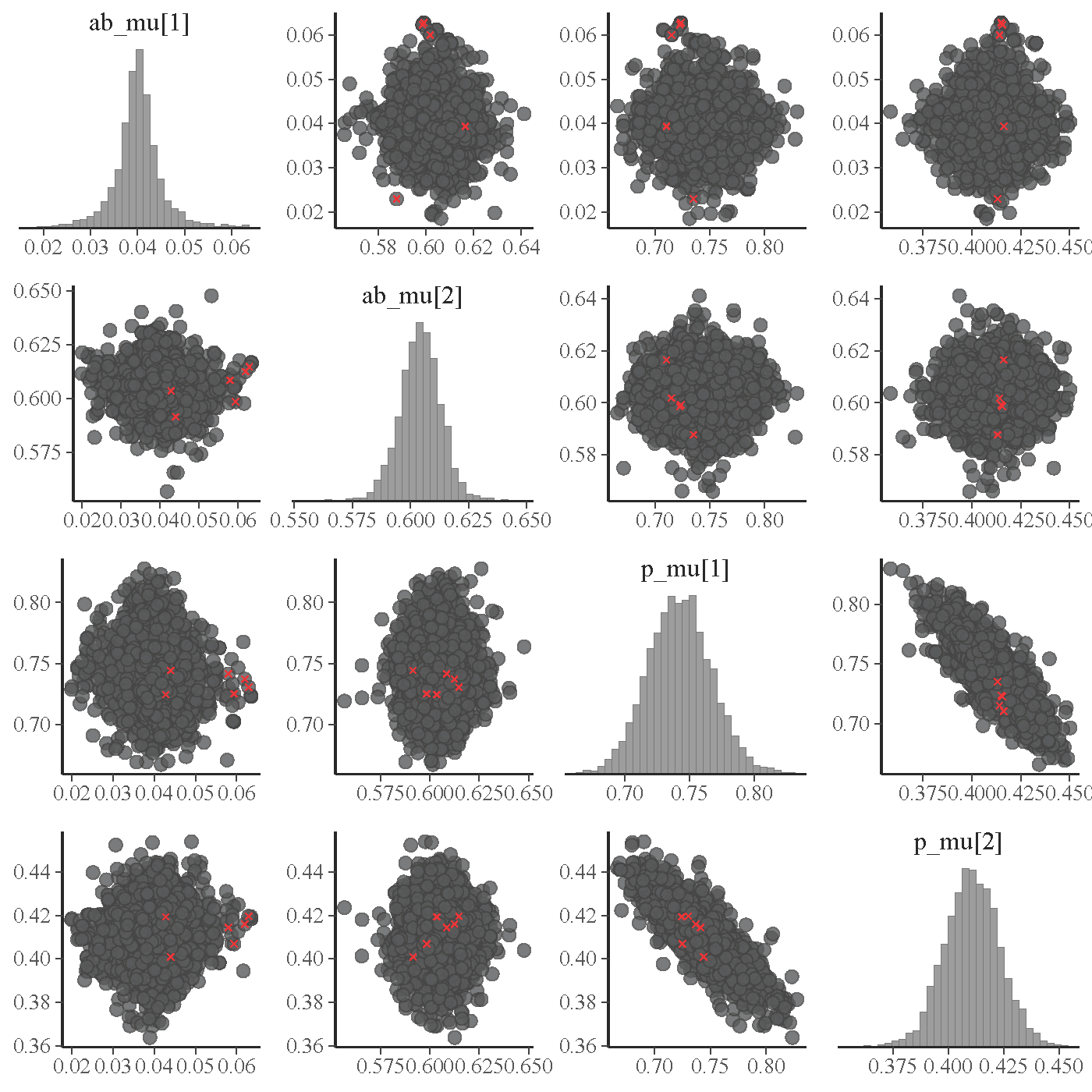
The first pairs plot above, based on 5,000 simulated observation points, shows that even after reparametrization, p_mu[1:2] are still rather highly correlated (although the p_err[1:2] are not and have nice pairs plots with other parameters in the model).

Q1: Is the high correlation between p_mu[1:2] problematic? If yes, what else can be done since they are already from the non-centered reparametrization of the original p[1:2]?

The first pairs plot also shows a distribution of ab_mu[1] with long and very thin tails. A divergent transition also happened in a tail. I guess these thin tails could be the cause of some unreliable estimates despite that the number of simulated observation points in that case was very large (14,000).

I tried some alternatives like specifying a tight prior but couldn’t easily get rid of the thin tails that seem to a cause of the not so accurate estimates. I also tried imposing an explicit constraint in declaring ab_mu[1]. This did not remove the suspected distortion but only resulted in a weird concentration of densities around the explicitly imposed boundaries.

Q2: Is there an effective way to get rid of the distorting thin tails (which actaully look like many extremely small local modes) if I have an intuitive reason to believe that the true parameters cannot be in those thin-tail regions?

The second pairs plot shows that even when the number of simulated observation points increases to 12,000 from 5,000, those issues remained and actually there were more divergent transitions (4 in this case and up to 12 in another occasion).

Q3: I ran 6 chains, 2000 iterations each, 1000 for warmup, so totally 6,000 draws for sampling. Given this, are 12 divergent transitions acceptable or even one is too many? Also, is there a way to obtain the estimates without the influence of the divergent transitions?

Below also shows true parameter values and the table of estimates based on 14,000 simulated observation points. While most of the estimates are rather close to the true values, w[1:2] seem to be still quite far off (underestimated by about 10% of the true values and also outside the 10-90 range). w together with g are already the transformed parameters of a joint non-centered reparametrization of them (so having a single covariance matrix).

Q4: Like p, w is the coefficient vector of a known covariate matrix G, where G*w is the input of an inv_logit() function. Is there anything that can be done to make the estimates of w highly accurate given such a model setup?

Would appreciate very much any advice. Many thanks.

#====================================================
# sd_y = 0.08, mu_u1 = 0.1; 
# mu_alpha = 0.04; beta = 0.6; theta = 0.15; 
# sd_season = 0.1, mu_season = c(-0.12, -0.06, 0.15);
# p = c(0.72, 0.42) 
# g = c(0.85, 0.35) 
# w = c(0.72, 0.15, 0.62)
# d = c(0.05, 0.7, 0.25)
#====================================================

observation points of simulated data: 140x100
6 chains, each with iter=2000; warmup=1000; thin=1;
post-warmup draws per chain=1000, total post-warmup draws=6000.

                   mean se_mean    sd    10%    50%    90% n_eff  Rhat

    sd_y          0.080   0.000 0.000  0.079  0.080  0.080  9126 1.000
    mu_u1         0.096   0.000 0.008  0.086  0.096  0.105  9032 1.000
    mu_alpha      0.041   0.000 0.001  0.039  0.041  0.042  5983 1.000
    beta          0.594   0.000 0.007  0.585  0.594  0.602  4472 1.000
    theta         0.146   0.000 0.005  0.140  0.146  0.152  6033 1.000
    sd_season     0.097   0.000 0.003  0.093  0.097  0.102  9910 1.000
    mu_season[1] -0.112   0.000 0.008 -0.122 -0.112 -0.102  8775 1.000
    mu_season[2] -0.060   0.000 0.008 -0.071 -0.060 -0.050 10503 0.999
    mu_season[3]  0.148   0.000 0.009  0.137  0.148  0.159  7612 1.000
    p[1]          0.697   0.000 0.021  0.671  0.697  0.724  6652 1.000
    p[2]          0.434   0.000 0.010  0.421  0.435  0.447  6156 1.000
    g[1]          0.870   0.000 0.037  0.823  0.870  0.918  7100 1.000
    g[2]          0.367   0.000 0.017  0.346  0.367  0.389  6608 1.000
    w[1]          0.801   0.001 0.050  0.737  0.801  0.865  5909 1.001
    w[2]          0.135   0.000 0.010  0.123  0.135  0.148  7461 1.001
    w[3]          0.623   0.000 0.017  0.601  0.623  0.645  7538 1.000
    d[1]          0.061   0.000 0.009  0.049  0.061  0.072  7564 1.000
    d[2]          0.688   0.000 0.008  0.678  0.688  0.698  7861 1.000
    d[3]          0.251   0.000 0.009  0.239  0.251  0.263  7831 1.000

I do not think the correlation in the posteriors you plotted would be enough to give the numerics difficulty.

It’s probably worth trying to do some exploratory plots or something to figure out why those tails are there. They must be reasonable-enough solutions that you’re sampling them frequently. Maybe make plots of predictions when this parameter is in the tail regions vs. not tail regions to try to see what is going on.

Have you tried adding control(adapt_delta = 0.99) as a way to get rid of divergences (Runtime warnings and convergence problems)?

Thanks for your feedback and advice. Appreciated. Just tried the control(adapt_delta = 0.99) option and it does result in no divergences.

You can probably make that lower and it’ll still work. The default is 0.8. The adapt_delta argument tells Stan to pick the timestep so that the estimated acceptance rate is adapt_delta. 0.99 is more conservative and encourages Stan to pick a smaller timestep. Ideally this gets rid of divergences but it’ll lead to slower inferences.

Thanks. Tried 0.9 and still with divergences; so trying 0.95 now.

I also extended p[1:2] in my model to p[1:3] (so the old p[1:2]= the new p[2:3] because the new p[1] – an intercept parameter – was previously hard-coded into the model). This changes the nature of the correlation between parameters: now between the mean non-centered parameters p_mu[1] and p_mu[3], as shown in the pairs plot below; previously between p_mu[2] and p_mu[3](ie, the then p_mu[1:2] before the extension).

Do you think I need to worry about the seemingly much stronger correlation in this extended model? And if yes, how to deal with it?

How many parameters do you have total?

Thanks for asking. Is it the exact number of the original parameters that you want to know?

Perhaps, I should outline the structure of the model components. Those shown in the estimation table in my post are all the original parameters:

(i) for the component of the state-space model of a latent AR(1) process,

  • mu_alpha, beta are the intercept and slope parameters of the AR(1) process
  • mu_u1 is the process’s initial value (when the time index n = 1)
  • mu_season and sd_season are the mean and sd of the seasonality component of the process (for quarterly data)
  • sd_y is the sd of the error term of the AR(1) process

(ii) laying on top of the state-space model are several sigmoid function components (either inv_logit() or a soft-clipping function) with inputs Z*p, X*g, and G*w (where p, g, w are unknown parameters and Z, X, G are known covariate matrices)

(iii) these sigmoid functions connect the latent process (y) to the observed process (r):

r = y + Real + D,

where

  • Real is a function of an unknown parameter theta and a sigmoid function of Z*p;
  • D is a function of an unknown simplex vector d and the multiplication of a sigmoid function of X*g with a sigmoid function of G*w.

With the non-centered reparametrization of p and (g,w) and (mu_alpha, beta), they become transformed parameters of p_mu, p_sd, p_L, p_err, gw_mu, gw_sd, …, ab_mu, ab_sd, …, etc that were not shown in the estimation table of my post (but shown in the pairs plot).

I have been struggling with better ways to get reliable estimates of p, g, and w (it is less challenging for other parameters).

  • If the intercept p[1] of Z*p is hard-coded into the model (note: Z[n,1] is a vector of 1's), it is easier to get reliable estimates of p[2:3], which are not so strongly correlated;
  • However, if all p[1:3] are free parameters to be estimated, there is very strong correlation between p[1] and p[3] as shown in the pairs plot in my last reply.

0.95 is sufficient to avoid any divergence and get reasonable estimates of the parameters with the following setup but the downside is that it took over 7 hours (for a fast machine on a cluster) to complete fitting the model.

Number of simulated observation points N = 12,000 (120 firms x 100 quarters)
4 chains, each with iter=3000; warmup=1000; thin=1;
post-warmup draws per chain=2000, total post-warmup draws=8000.

True parameter values:
====================================================
sd_y = 0.08, mu_u1 = 0.1; mu_alpha = 0.04; beta = 0.6;  
theta = 0.15;  
sd_season = 0.1, mu_season = c(-0.12, -0.06, 0.15); 
p = c(0.7, 0.62, 0.35) 
g = c(0.85, 0.35)  
w = c(0.72, 0.15, 0.62)  
d = c(0.05, 0.7, 0.25) 
====================================================

               mean se_mean    sd    10%    50%    90% n_eff  Rhat
sd_y          0.080   0.000 0.001  0.079  0.080  0.080 15212 1.000
mu_u1         0.095   0.000 0.008  0.084  0.095  0.105 12897 1.000
mu_alpha      0.041   0.000 0.002  0.039  0.041  0.043  6549 1.000
beta          0.587   0.000 0.007  0.578  0.587  0.597  4486 1.000
theta         0.152   0.000 0.008  0.142  0.152  0.163  6515 1.000
sd_season     0.102   0.000 0.004  0.097  0.102  0.107 12263 1.000
mu_season[1] -0.122   0.000 0.010 -0.135 -0.122 -0.110 14662 1.000
mu_season[2] -0.054   0.000 0.009 -0.066 -0.054 -0.042 16905 1.000
mu_season[3]  0.155   0.000 0.009  0.143  0.155  0.167 14127 1.000
p[1]          0.712   0.001 0.043  0.670  0.704  0.764  2432 1.002
p[2]          0.614   0.000 0.026  0.581  0.613  0.647 11231 1.000
p[3]          0.371   0.001 0.061  0.311  0.357  0.446  2405 1.002
g[1]          0.872   0.000 0.041  0.818  0.871  0.925  7061 1.000
g[2]          0.350   0.000 0.018  0.327  0.350  0.373  6253 1.000
w[1]          0.670   0.001 0.056  0.598  0.671  0.741  5806 1.000
w[2]          0.158   0.000 0.011  0.144  0.158  0.172  8606 1.000
w[3]          0.621   0.000 0.018  0.598  0.620  0.644  9303 1.000
d[1]          0.050   0.000 0.009  0.039  0.050  0.062  9629 1.000
d[2]          0.687   0.000 0.008  0.677  0.687  0.698 16379 1.000
d[3]          0.262   0.000 0.010  0.250  0.262  0.275  9252 1.000

So it looks like this model has 20 some parameters?

Maybe try adding control(metric = “dense_e”) and see if that helps?

Also, are your lowest Neffs 2000~? You might consider just running your calculations a shorter amount of time if so.

Can you run get_num_leapfrog_per_iteration(fit) on your fit?

Thanks for suggesting the metric = "dense_e" option. Tried but it doesn’t seem to work in this case: still at the very early stage of warmup after 15 hours of fitting.

If I understand correctly, the considerations related to the metric = "dense_e" option are discussed on this page. I include the link here in case others reading this post want to consider the option.

I don’t think the fix for the dense metric has made it into the rstan on CRAN yet…

2 Likes

Thanks for the suggestions. Tried 1500 iterations (with 1000 warmups for 4 chains for simulated obs. N = 120 firms x 100 quarters). The lowest neff dropped to only around 340 (from previously 2000+ when running 3000 iterations with 1000 warmups for 4 chains).

Despite the large reduction in the number of iterations and the neff, the fitting time only dropped to 5.5 hours (from over 7 hours). Running get_num_leapfrog_per_iteration(fit) gives

   [1] 255 511 255 255 511 255 255 511 511 255 511 511 511 511 255 255 511 511
  [19] 511 255 511 255 255 511 255 255 255 511 255 255 255 511 255 255 511 255
  [37] 255 255 511 511 511 511 511 511 255 511 511 511 511 255 255 511 511 511
  [55] 511 255 255 255 511 511 511 511 255 511 511 255 511 511 511 511 511 511
  ... (others omitted)

Q: For a complex model like this, is a fitting time of 5.5 hours considered uncommonly long? (I am aware of the benefit of vectorization and have implemented it wherever I see possible.)

I also tried 2000 iterations (with 1000 warmups for 4 chains for simulated obs. N = 60 firms x 100 quarters). The lowest neff for the hard-to-estimate p[1] and p[3] are around 1800. get_num_leapfrog_per_iteration(fit) returns 255 255 255 ... consistently.

The fitting time for this case is a more realistic 2 hours. Previously, I focused on 120 firms because with only 60 firms, usually one of the estimates tends to be not so accurately estimated. For example, the true value of d[1] should be 0.05 but its estimate is 0.072 and the 10-90 interval does not contain the true value (see the table below).

Q: In the tradition of Bayesian analysis, is such a case with an exception or two of not so accurate estimates still considered a good enough validation of the model to justify using it to look at real data? (eg, for industries with at least 60 firms)

               mean se_mean    sd    10%    50%    90% n_eff  Rhat
sd_y          0.079   0.000 0.001  0.078  0.079  0.080  5479 1.000
mu_u1         0.099   0.000 0.011  0.085  0.099  0.113  4435 1.001
mu_alpha      0.037   0.000 0.002  0.034  0.037  0.040  3733 1.000
beta          0.599   0.000 0.010  0.586  0.599  0.613  2076 1.002
theta         0.149   0.000 0.011  0.136  0.148  0.162  2912 1.001
sd_season     0.099   0.000 0.005  0.092  0.099  0.106  3922 1.000
mu_season[1] -0.116   0.000 0.013 -0.133 -0.116 -0.099  5608 1.000
mu_season[2] -0.066   0.000 0.013 -0.083 -0.065 -0.049  6569 1.000
mu_season[3]  0.144   0.000 0.013  0.128  0.144  0.161  5244 1.000
p[1]          0.756   0.001 0.063  0.690  0.743  0.845  1807 1.004
p[2]          0.643   0.001 0.040  0.593  0.642  0.694  4613 0.999
p[3]          0.423   0.002 0.091  0.328  0.403  0.552  1756 1.003
g[1]          0.841   0.001 0.055  0.770  0.840  0.910  2883 1.001
g[2]          0.349   0.000 0.025  0.317  0.349  0.381  3179 1.000
w[1]          0.710   0.002 0.078  0.611  0.710  0.809  2514 1.000
w[2]          0.158   0.000 0.015  0.139  0.158  0.178  3523 1.000
w[3]          0.618   0.000 0.025  0.585  0.618  0.651  3438 1.002
d[1]          0.072   0.000 0.014  0.055  0.073  0.090  4029 0.999
d[2]          0.711   0.000 0.012  0.695  0.711  0.726  8837 0.999
d[3]          0.216   0.000 0.014  0.198  0.217  0.235  3623 1.000

is a fitting time of 5.5 hours considered uncommonly long?

It’s more about the number of gradient evaluations than total walltime. It looks like your chains are taking 255+ leapfrog steps before hitting a U-turn. That is a lot.

If you have a relatively modest number of parameters (is it actually just 20?) then dense adaptation might help, but like @Charles_Driver said there was a bug (and a bugfix) that may not have actually propagated to the released rstan yet. If you have the patience, you might try running this model with cmdstan.

If you have hundreds of parameters though, this probably wouldn’t work so easily. So the number is important, smaller is easier.

It sounds like the model is sampling really efficiently, it’s just taking a lot of leapfrog steps to do it. I think give cmdstan dense adaptation a try.

If you want to dump data constructed for rstan into a format that cmdstan can read (assuming you have that data in a list called ‘data’), use:

stan_rdump(names(data), file = "mydata.dat", list2env(data))
1 Like

originally 20 but after non-centered reparametrization of the correlated parameters, the total number of raw parameters to sample becomes 78.

Thanks for the guidance. Tried this but got the error message:

objects not found: r, Z, X, G
Error in as.logical(test) : cannot coerce type 'environment' to vector of type 'logical'

Confused because those objects (r, Z, X, G) are clearly in my environment. (r is a list of vectors and Z, X, G are lists of matrices, both as declared in the .stan file.)
Any idea on the error message?

Oh whoops, my bad, that last argument should be named:

stan_rdump(names(data), file = "mydata.dat", envir = list2env(data))

And this is assume that data is a list like:

data = list(N = ...,
            y = ...,
            ...)

(The thing you’d pass into a Stan sampling statement).

78 parameters should be fine for this.

Thanks for the clarification. I successfully stan_rdump() the data. In installing cmdstan, I successfully completed the make build step. However, when compiling the .stan file (which I have been using with rstan without a problem), I received the errors below. In another (slower) cluster, I could complete this step and proceed to sampling without a problem.

Any idea on how to fix the compliation errors? (Are they due to the g++ version, which is g++ (GCC) 4.8.5 20150623 (Red Hat 4.8.5-36)?)

[sbbg070@wrds-cloud-login1-h ~/cmdstan-2.19.1]$ make ../SSM0.5.2dev

--- Translating Stan model to C++ code ---
bin/stanc  --o=../SSM0.5.2dev.hpp ../SSM0.5.2dev.stan
Model name=SSM0_5_2dev_model
Input file=../SSM0.5.2dev.stan
Output file=../SSM0.5.2dev.hpp
DIAGNOSTIC(S) FROM PARSER:
Info: Comments beginning with # are deprecated.  Please use // in place of # for line comments.
Info:
Left-hand side of sampling statement (~) may contain a non-linear transform of a parameter or local variable.
If it does, you need to include a target += statement with the log absolute determinant of the Jacobian of the transform.
Left-hand-side of sampling statement:
    err_y[j] ~ normal(...)

g++ -std=c++1y -pthread -Wno-sign-compare     -O3 -I src -I stan/src -I stan/lib/stan_math/ -I stan/lib/stan_math/lib/eigen_3.3.3 -I stan/lib/stan_math/lib/boost_1.69.0 -I stan/lib/stan_math/lib/sundials_4.1.0/include    -DBOOST_RESULT_OF_USE_TR1 -DBOOST_NO_DECLTYPE -DBOOST_DISABLE_ASSERTS -DBOOST_PHOENIX_NO_VARIADIC_EXPRESSION     -c -MT ../SSM0.5.2dev.o -MT ../SSM0.5.2dev -include ../SSM0.5.2dev.hpp -include src/cmdstan/main.cpp -MM -E -MG -MP -MF ../SSM0.5.2dev.d ../SSM0.5.2dev.hpp

--- Linking C++ model ---
g++ -std=c++1y -pthread -Wno-sign-compare     -O3 -I src -I stan/src -I stan/lib/stan_math/ -I stan/lib/stan_math/lib/eigen_3.3.3 -I stan/lib/stan_math/lib/boost_1.69.0 -I stan/lib/stan_math/lib/sundials_4.1.0/include    -DBOOST_RESULT_OF_USE_TR1 -DBOOST_NO_DECLTYPE -DBOOST_DISABLE_ASSERTS -DBOOST_PHOENIX_NO_VARIADIC_EXPRESSION             -include ../SSM0.5.2dev.hpp src/cmdstan/main.cpp        stan/lib/stan_math/lib/sundials_4.1.0/lib/libsundials_nvecserial.a stan/lib/stan_math/lib/sundials_4.1.0/lib/libsundials_cvodes.a stan/lib/stan_math/lib/sundials_4.1.0/lib/libsundials_idas.a  -o ../SSM0.5.2dev
In file included from stan/lib/stan_math/stan/math/rev/mat/fun/ordered_constrain.hpp:6:0,
                 from stan/lib/stan_math/stan/math/rev/mat.hpp:41,
                 from stan/lib/stan_math/stan/math.hpp:4,
                 from stan/src/stan/model/model_header.hpp:4,
                 from ./../SSM0.5.2dev.hpp:3,
                 from <command-line>:0:
stan/lib/stan_math/stan/math/rev/mat/functor/adj_jac_apply.hpp:31:32: error: ‘std::index_sequence’ has not been declared
                           std::index_sequence<I...> i) {
                                ^
stan/lib/stan_math/stan/math/rev/mat/functor/adj_jac_apply.hpp:31:46: error: expected ‘,’ or ‘...’ before ‘<’ token
                           std::index_sequence<I...> i) {
                                              ^
stan/lib/stan_math/stan/math/rev/mat/functor/adj_jac_apply.hpp: In function ‘constexpr auto stan::math::internal::apply(const F&, const Tuple&)’:
stan/lib/stan_math/stan/math/rev/mat/functor/adj_jac_apply.hpp:49:27: error: ‘make_index_sequence’ is not a member of ‘std’
   return apply_impl(f, t, std::make_index_sequence<std::tuple_size<Tuple>{}>{});
                           ^
stan/lib/stan_math/stan/math/rev/mat/functor/adj_jac_apply.hpp:49:27: note: suggested alternative:
In file included from stan/lib/stan_math/lib/boost_1.69.0/boost/fusion/container/vector/vector.hpp:28:0,
                 from stan/lib/stan_math/lib/boost_1.69.0/boost/fusion/container/vector/vector10.hpp:25,
                 from stan/lib/stan_math/lib/boost_1.69.0/boost/fusion/view/transform_view/transform_view.hpp:22,
                 from stan/lib/stan_math/lib/boost_1.69.0/boost/fusion/algorithm/transformation/transform.hpp:11,
                 from stan/lib/stan_math/lib/boost_1.69.0/boost/fusion/view/zip_view/detail/begin_impl.hpp:14,
                 from stan/lib/stan_math/lib/boost_1.69.0/boost/fusion/view/zip_view/zip_view.hpp:16,
                 from stan/lib/stan_math/lib/boost_1.69.0/boost/fusion/view/zip_view.hpp:12,
                 from stan/lib/stan_math/lib/boost_1.69.0/boost/fusion/include/zip_view.hpp:11,
                 from stan/lib/stan_math/lib/boost_1.69.0/boost/numeric/odeint/util/resize.hpp:26,
                 from stan/lib/stan_math/lib/boost_1.69.0/boost/numeric/odeint/util/state_wrapper.hpp:26,
                 from stan/lib/stan_math/lib/boost_1.69.0/boost/numeric/odeint/util/ublas_wrapper.hpp:33,
                 from stan/lib/stan_math/lib/boost_1.69.0/boost/numeric/odeint.hpp:25,
                 from stan/lib/stan_math/stan/math/prim/arr/functor/integrate_ode_rk45.hpp:17,
                 from stan/lib/stan_math/stan/math/prim/arr.hpp:46,
                 from stan/lib/stan_math/stan/math/prim/mat.hpp:344,
                 from stan/lib/stan_math/stan/math/rev/mat.hpp:12,
                 from stan/lib/stan_math/stan/math.hpp:4,
                 from stan/src/stan/model/model_header.hpp:4,
                 from ./../SSM0.5.2dev.hpp:3,
                 from <command-line>:0:
stan/lib/stan_math/lib/boost_1.69.0/boost/fusion/support/detail/index_sequence.hpp:59:12: note:   ‘boost::fusion::detail::make_index_sequence’
     struct make_index_sequence
            ^
In file included from stan/lib/stan_math/stan/math/rev/mat/fun/ordered_constrain.hpp:6:0,
                 from stan/lib/stan_math/stan/math/rev/mat.hpp:41,
                 from stan/lib/stan_math/stan/math.hpp:4,
                 from stan/src/stan/model/model_header.hpp:4,
                 from ./../SSM0.5.2dev.hpp:3,
                 from <command-line>:0:
stan/lib/stan_math/stan/math/rev/mat/functor/adj_jac_apply.hpp:49:77: error: expected primary-expression before ‘{’ token
   return apply_impl(f, t, std::make_index_sequence<std::tuple_size<Tuple>{}>{});
                                                                             ^
stan/lib/stan_math/stan/math/rev/mat/functor/adj_jac_apply.hpp:49:77: error: expected ‘)’ before ‘{’ token
stan/lib/stan_math/stan/math/rev/mat/functor/adj_jac_apply.hpp: At global scope:
stan/lib/stan_math/stan/math/rev/mat/functor/adj_jac_apply.hpp:151:9: error: expected type-specifier
       = std::result_of_t<F(decltype(is_var_), decltype(value_of(Targs()))...)>;
         ^
stan/lib/stan_math/stan/math/rev/mat/functor/adj_jac_apply.hpp:156:42: error: ‘FReturnType’ was not declared in this scope
   std::array<int, internal::compute_dims<FReturnType>::value> M_;
                                          ^
stan/lib/stan_math/stan/math/rev/mat/functor/adj_jac_apply.hpp:156:53: error: template argument 1 is invalid
   std::array<int, internal::compute_dims<FReturnType>::value> M_;
                                                     ^
stan/lib/stan_math/stan/math/rev/mat/functor/adj_jac_apply.hpp:156:61: error: template argument 2 is invalid
   std::array<int, internal::compute_dims<FReturnType>::value> M_;
                                                             ^
stan/lib/stan_math/stan/math/rev/mat/functor/adj_jac_apply.hpp: In member function ‘std::vector<stan::math::var> stan::math::adj_jac_vari<F, Targs>::build_return_varis_and_vars(const std::vector<double>&)’:
stan/lib/stan_math/stan/math/rev/mat/functor/adj_jac_apply.hpp:349:9: error: invalid types ‘int[int]’ for array subscript
     M_[0] = val_y.size();
         ^
stan/lib/stan_math/stan/math/rev/mat/functor/adj_jac_apply.hpp:350:32: error: invalid types ‘int[int]’ for array subscript
     std::vector<var> var_y(M_[0]);
                                ^
stan/lib/stan_math/stan/math/rev/mat/functor/adj_jac_apply.hpp: In member function ‘Eigen::Matrix<stan::math::var, R, C> stan::math::adj_jac_vari<F, Targs>::build_return_varis_and_vars(const Eigen::Matrix<double, R, C>&)’:
stan/lib/stan_math/stan/math/rev/mat/functor/adj_jac_apply.hpp:375:9: error: invalid types ‘int[int]’ for array subscript
     M_[0] = val_y.rows();
         ^
stan/lib/stan_math/stan/math/rev/mat/functor/adj_jac_apply.hpp:376:9: error: invalid types ‘int[int]’ for array subscript
     M_[1] = val_y.cols();
         ^
stan/lib/stan_math/stan/math/rev/mat/functor/adj_jac_apply.hpp:377:40: error: invalid types ‘int[int]’ for array subscript
     Eigen::Matrix<var, R, C> var_y(M_[0], M_[1]);
                                        ^
stan/lib/stan_math/stan/math/rev/mat/functor/adj_jac_apply.hpp:377:47: error: invalid types ‘int[int]’ for array subscript
     Eigen::Matrix<var, R, C> var_y(M_[0], M_[1]);
                                               ^
stan/lib/stan_math/stan/math/rev/mat/functor/adj_jac_apply.hpp: In member function ‘void stan::math::adj_jac_vari<F, Targs>::chain( ’:
stan/lib/stan_math/stan/math/rev/mat/functor/adj_jac_apply.hpp:530:5: error: ‘FReturnType’ was not declared in this scope
     FReturnType y_adj;
     ^
stan/lib/stan_math/stan/math/rev/mat/functor/adj_jac_apply.hpp:530:17: error: expected ‘;’ before ‘y_adj’
     FReturnType y_adj;
                 ^
stan/lib/stan_math/stan/math/rev/mat/functor/adj_jac_apply.hpp:532:38: error: ‘y_adj’ was not declared in this scope
     internal::build_y_adj(y_vi_, M_, y_adj);
                                      ^
stan/lib/stan_math/stan/math/rev/mat/functor/adj_jac_apply.hpp:536:26: error: expansion pattern ‘auto&&’ contains no argument packs
         [this](auto&&... args) { this->accumulate_adjoints(args...); },
                          ^
stan/lib/stan_math/stan/math/rev/mat/functor/adj_jac_apply.hpp: In lambda function:
stan/lib/stan_math/stan/math/rev/mat/functor/adj_jac_apply.hpp:536:60: error: ‘args’ was not declared in this scope
         [this](auto&&... args) { this->accumulate_adjoints(args...); },
                                                            ^
make: *** [../SSM0.5.2dev] Error 1

Also, I followed p.28 of the cmdstan-guide-2.19.1.pdf to hope to sample 4 chains in parallel but the chains ran sequentially even when multiple cores are specified.

Any suggestion or pointer to the correct commands for a cluster environment?

#PBS -l nodes=1:ppn=8

for i in {1..4}
do
../SSM0.5.2dev sample algorithm=hmc metric=dense_e adapt delta=0.95 \
id=$i data file=../SSM_data.dat output file=samples$i.csv 
done

Did you get things to compile? I’m guessing this is the compiler. I think Stan supports gcc 4.9.3 (whatever Rtools is at). std::index_sequence is a c++14 thing (https://en.cppreference.com/w/cpp/utility/integer_sequence)

To do four chains in parallel, you gotta run four separate things. If I remember correct qsub scripts just launch the same script on however many different nodes you request, so maybe just do something like:

#PBS

../SSM0.5.2dev sample algorithm=hmc metric=dense_e adapt delta=0.95 \
id=$PBS_ARRAYID data file=../SSM_data.dat output file=samples$PBS_ARRAYID.csv

And then however many nodes you request via qsub (or cores or however it’s denoted), you’ll get that many outputs. Use the examples/bernoulli job to test this.

1 Like

Hi, Ben:

I finally completed a run of 4 chains using metric=dense_e (to compare with that using metric=diag_e). It does reduce the run time significantly (with essentially the same estimates given the large amount of simulated data used: 12,000 data points).
Here are the summary output: dense_e_cmdStan0.5.2dev_2.6hrs.txt (5.2 KB) diag_e_cmdStan0.5.2dev_9.6hrs.txt (5.2 KB)

Would appreciate very much your feedback on whether there’s anything that I should pay attention to, especially about the diagnostic indicators. Thanks.

1 Like

Well the things to watch out for are the usual things: are there divergences in the dense_e version and are the Rhats 1?

Your N_effs still seem really high. You might be able to get away with cutting your chain lengths in half or something. Maybe try 500 warmup/500 samples and see what happens? I wouldn’t go much less than 500 though. Each chain needs to be long enough to do warmup and get enough N_eff individually to make the Rhats and such reliable.

1 Like