Not good results with projpred

Hi everyone!

I have been working with the projpred package lately and I don’t feel very confident with the results. I started using stepwise regression when I found this package, and I think is the tool I need. I have 39 variables/features (x1,x2,x3,…,x39) and I want to reproduce the response variable y. My prior knowledge is that some of the variables may be not relationated with y, and some of them are highly correlationated with the others, so the information the carry is redundant. The idea is then to find a minimal subset of the variables to reproduce the y value.

I tried with the horseshoe prior as indicated by Piironen and Vehtari (2017):

formula <- y ~ x1 + x2 + x3 + x4 + x5 + x6 + x7 + x8 + x9 + x10 + x11 + x12 + x13 + x14 + x15 + x16 + x17 + x18 + x19 + x20 + x21 + x22 + x23 + x24 + x25 + x26 + x27 + x28 + x29 + x30 + x31 + x32 + x33 + x34 + x35 + x36 + x37 + x38 + x39
n <- nrow(data)
D <- 39 # number of parameters
p0 <- 15 # prior guess for the number of relevant variables
tau0 <- p0/(D-p0) * 1/sqrt(n) 
fit <- brm(formula, family=gaussian(), data=data,
           prior=prior(horseshoe(scale_global = tau0, scale_slab = 1), class=b),
           seed=123456789, chains=4, iter=2000, warmup=1000,
           control=list(max_treedepth=12,adapt_delta=0.99), save_pars=save_pars(all=TRUE))

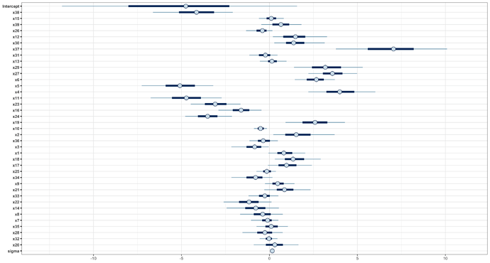
The results, with mcmc_intervals, are:


(the order of the variables is the one got by cv_varsel, see later) Note the high dispersion/error on the Intercept. This is a problem I think, since the range of my response variable is range(y) = [-1.58 , 0.37], so I don’t know if I can be confident about the predictions for y with that uncertainty.

Let’s go to proper projpred. I construct the reference model and use the cv_varsel function:

refmodel <- get_refmodel(fit)
vs <- cv_varsel(refmodel, method = "forward", nterms_max = 50)
plot(vs, stats = c('elpd', 'rmse'))

vsplot
I get this plot, and using the suggest_size function with ‘elpd’ or ‘rmse’, it suggests me to use 19 variables. So, now:

proj <- project(vs, nterms = 19, ns = 500)
mcmc_intervals(as.matrix(proj))


The Intercept has a large dispersion again, and some of the coefficients (x31, x13) are nearly zero! I don’t feel very confident about this.

Finally, I plot the predictions using the reference model (blue x) and the submodel (black dots) versus the original y values, with the 1:1 relationship:
pred_y
So it seems like projpred did a good job, reproducing with the submodel the predictions of the reference model. But I think it could be better, with less dispersion (i.e. the predictions closer to the 1:1 line), and better coefficients (that is, less dispersion for the intercept, coeffs nearly zero?, etc.)

Does someone know if I can do better? May be a problem with the reference model?
Well, projpred compares the predictive distributions of a reduced model and a reference one, where the reference model is a full model you might believe is correct, so if you already know there are strongly correlated variables, would not be better to eliminate them from the reference model? Probably you would have better results like that but is better if a projpred expert helps you with it (@AlejandroCatalina ).

Asael did have good points already. Projpred can only work with whatever is present in the reference model. On top of that, projpred focuses on explaining the predictions, and therefore the projected posterior margínala are not necessarily well calibrated, which I believe is your intuition. The question that projpred answers is rather “which variables are sufficient to explain the predictions of the reference model?”.

You can try setting more informative priors (horseshoe is a good start, but how much did you elaborate its parameters?) and see how that translates to the projection.

Hope this was helpful!

Thanks @asael_am and @AlejandroCatalina for your comments!

Okey, so it seems like I need to improve my reference model first to apply then projpred. As some variables are strongly correlated (for example, x7 and x9 has a correlation of 0.99, and a lot of them has correlations over 0.85), how I decide which variable should be eliminated? Should a choose a threshold in the correlation, and eliminate the variables with higher correlation following the order given above? For example, I should keep x9 and delete x7 because it appears first in my first plot above. Or should I apply other criterion, like fitting the model twice, once keeping one variable and once the other, and then choosing the model with higher elpd? Is there a way to include the correlations between variables in the model to implement all of this?

About the priors, how can I make them more informative? I am new with the horseshow priors, and I elaborated the parameters as explained in the documentation and some of the papers, but I don’t know much more can I do.

As you said, the question that projpred answers is “which variables are sufficient to explain the predictions of the reference model?”. So, could I create a ‘fake’ reference model as

formula <- y ~ x1 + x2 + x3 + x4 + x5 + x6 + ... + x39 + y

so the coefficients will be zero for all x’s and 1 for y, then the reference model will be a ‘perfect model’ that reproduces exactly the response variable, and I can apply projpred to choose which variables (not including y) can reproduce well the ‘reference model’. My intuition is that this must not be done, but I think it is worth asking, just in case.

Thank you again!

It looks like you predictors might have very different variances which makes the interpretation of the marginal effect plots more difficult. This is illustrated in the first plot in Regression and Other Stories: Student

If the prior guess is almost half of the total number of variables, then RHS is not a useful prior. I would expect that by scaling the predictors and scaling with the number of covariates as discussed in Regression and Other Stories: Student would give you better results. I guess the difference would be small, but at least the computation would be faster and interpretation easier. Even better would be a prior that would take into account the very high correlations, but right now there is no direct solution for that in brms. For highly correlated variables you could try making the reference model with supervised PCA as in Projective inference in high-dimensional problems: Prediction and feature selection; but if the number of observations is much larger than the number of predictors then again the difference is likely to be small.