Context
I’m attempting to determine the influence of 7 covariates on a binary response variable with a Bayesian GLMM (using the excellent brms package). The dataset is unavoidably small (~200 observations). I’m afraid I can’t share the data here.
Following advice (e.g. https://cran.r-project.org/web/packages/loo/vignettes/loo2-weights.html; Piironen and Vehtari 2017), I’m using horseshoe priors to identify the most relevant covariates. [I’d like to use `projpred`, but am currently unable to because `projpred` doesn’t currently handle the random variables in my model (see https://github.com/stan-dev/projpred/issues/57).]
Problem
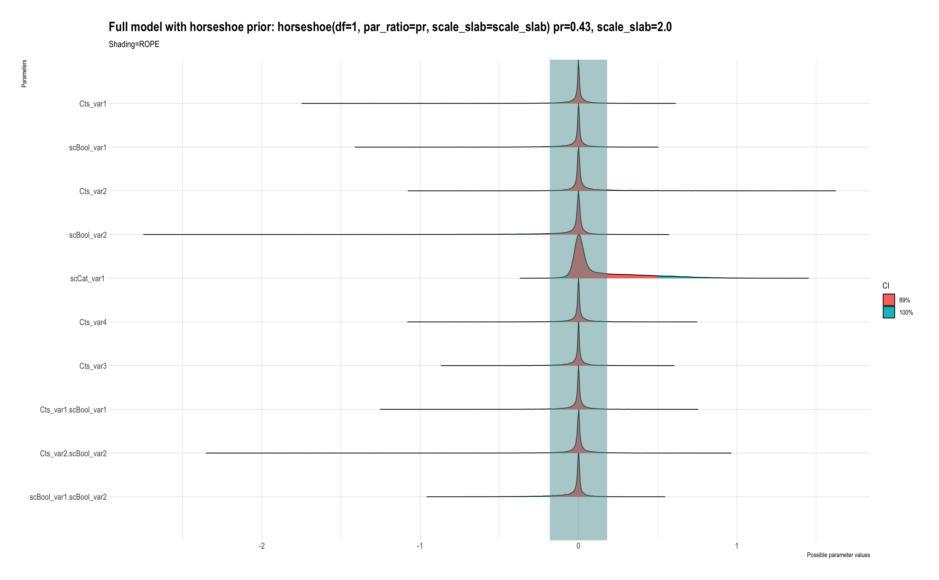
When using the regularised horseshoe prior, all of the predictors have negligible effect sizes. I understand that this is likely because there aren’t any strong effects which can be discerned from this small dataset. However, when using a weakly informative prior or frequentist models, there are relevant predictors. I would like to use the horseshoe prior to identify the most important ones, but it appears that its imposing too much shrinkage to be useful. I have tried adjusting the shrinkage using par_ratio in horseshoe{brms}, but to no avail.
The model with the horseshoe prior does fit the data better, however (see Stacking weights below).
I’d be grateful for any suggestions on how best to proceed with this variable selection; or if anyone can point out my error or misunderstanding. Am I forced to conclude that none of the predictors are important, even though the data exploration suggests not! My datasets will always be small, so I’m keen to identify the most appropriate Bayesian method for these data.
This is similar to How to make the regularized horseshoe less strict?
Many thanks in advance for your help.

Model
# Weakly informative prior (https://github.com/stan-dev/stan/wiki/Prior-Choice-Recommendations)
prior1 <-  c(set_prior("student_t(3,0,2)", class = "b"))

# Regularised horseshoe prior:
priorhs <- set_prior("horseshoe(df=1, par_ratio=3/7, scale_slab=2)", class='b')

# All predictors scaled to 0,1
# Have also scaled the categorical and boolean variables for the horseshoe prior model:
data$scBool_var1 <- scale(data$Bool_var1, center=T, scale=T)
data$scBool_var2 <- scale(data$Bool_var2, center=T, scale=T)
data$scCat_var1 <- scale(data$Cat_var1, center=T, scale=T)

# Formulae:

cfull_formula <- as.formula(y ~  Cts_var1 * Bool_var1 + Cts_var2 * Bool_var2 + Bool_var1:Bool_var2 + Cat_var1 + Cts_var3 + Cts_var4 + (1|rand1) + (1|rand2) + (1|rand3) )

cfull_formula_hs <- as.formula(y ~  Cts_var1 * scBool_var1 + Cts_var2 * scBool_var2 + scBool_var1:scBool_var2 + scCat_var1 + Cts_var3 + Cts_var4 + (1|rand1) + (1|rand2) + (1|rand3) )

# Models:

brms_cfull <- brm(cfull_formula, data=data, family="bernoulli", iter=10000, prior =  prior1,  sample_prior = T, control=list(adapt_delta=0.999,max_treedepth = 15), save_all_pars = F, refresh=0)

brms_cfull_hs <- brm(cfull_formula_hs, data=data, family="bernoulli", iter=10000, prior =  priorhs,  sample_prior = T, control=list(adapt_delta=0.999,max_treedepth = 15), save_all_pars = F, refresh=0)
Model weights
try(loo_model_weights(brms_cfull, brms_cfull_hs, method='stacking', model_names=c('brms_cfull', 'brms_cfull_hs')))

Method: stacking
------
              weight
brms_cfull    0.116
brms_cfull_hs 0.884
References
Piironen, J., and Vehtari, A. (2017). Sparsity information and regularization in the horseshoe and other shrinkage priors. https://arxiv.org/abs/1707.01694

