Trouble implementing GP regression with a spectral mixture kernel

Hi everyone.

I’ve been doing some messing around with the spectral mixture kernel for GP regression. I’ve tried to implement this kernel in Stan, and I’m wondering why I’m struggling to replicate the authors’ results on one of their synthetic examples.

If I’m to attempt a very brief introduction, the spectral mixture kernel aims to represent a stationary covariance structure in terms of its spectral density, which is approximated using a mixture of Q Gaussians.

Expressed in terms of \tau = x_1 - x_2, the kernel itself is:

k(\tau) = \displaystyle\sum_{q=1}^{Q} w_q \exp{(-2 \pi^2 \tau^2\nu_q ) } \cos{(2 \tau \pi \mu_q )}

where the (hyper-)parameters, \mu_q and \nu_q, respectively represent the mean and variance of each of the Q components of the Gaussian mixture used to approximate the spectral density. The weights, w_q, represent the relative contribution of each mixture component.

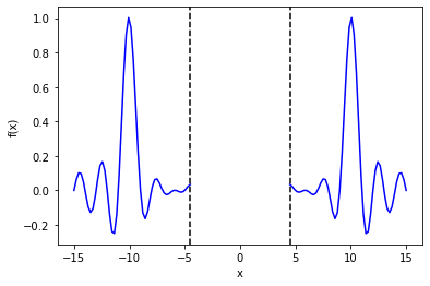
I’m trying to replicate the authors’ example on the “sinc” function, implemented in python as follows:

import numpy as np
sinc = lambda x: np.sin(np.pi * x) / (np.pi * x)
func = lambda x: sinc(x + 10) + sinc(x) + sinc(x - 10)

n = 300
x = np.concatenate([
    np.linspace(-15, -4.5, int(n/2)), 
    np.linspace(4.5, 15, int(n/2))]
)
y = func(x)

The aim is to predict the value of the function between -4.5 and 4.5, given data outside of this region:

image

My (rather crude) Stan model is:

functions {
  matrix L_cov_sm(vector x, vector mu, vector nu, vector w, real jitter, int N, int Q) {
    matrix[N, N] C;
    real tau;
    real tmp;
    for (i in 1:N){
      for (j in 1:i){
          tau = abs(x[i] - x[j]);
          tmp = 0;
          for (q in 1:Q){
              tmp += w[q] * exp(-2 * square(pi()) * square(tau) * nu[q]) * cos(2 * tau * pi() * mu[q]);
          }
          if (i == j) {tmp += jitter;}
          C[i, j] = tmp;
          C[j, i] = tmp; 
       }
      }
    return cholesky_decompose(C);
  }
}
data {
  int<lower=1> N;
  int<lower=1> Q;
  vector[N] x;
  vector[N] y;
  real<lower=0> jitter;
}
parameters {
  vector<lower=0>[Q] nu;
  vector[Q] mu;
  vector<lower=0>[Q] w;
}
transformed parameters {
  matrix[N, N] L;
  vector[N] meanv;
  L = L_cov_sm(x, mu, nu, w, jitter, N, Q);
  meanv = rep_vector(0, N);
}
model {
  w ~ cauchy(0, 5);
  mu ~ cauchy(0, 5);
  nu ~ normal(0, 1);
  y ~ multi_normal_cholesky(meanv, L);
}

Which, for the sake of providing a complete example, I’m running through pystan using:

import pystan
import multiprocessing
multiprocessing.set_start_method("fork")
Q = 10
data = {
    'x': x,
    'y': y, 
    'N': x.shape[0],
    'Q': Q,
    'jitter': 1e-10,
}
ret = smgp_sm.optimizing(data) # the model from before

As far as I can tell, the authors do not discuss prior distributions for any of the kernel parameters (the distributions for \mu, \nu and w you’re seeing in my model are an attempt to get the optimiser to behave better, though I suspect they’re still too vague to have much – if any – influence), and use gradient based optimisation to maximise the log likelihood.

I’ve been attempting to do the same using Stan’s optimiser.

I am occasionally getting sensible looking results using (the default) l-bfgs, and less occasionally getting sensible results using method='Newton'. I’m unsure whether the inconsistency I’m experiencing is due to just initialisation or initialisation and some kind of modelling error somewhere, as even when the posterior predictive distribution of the GP looks “about right” (I can include the code I use to do this if it’s valuable, but it’s pretty generic GP regression stuff), my values for \mu do not match the authors’.

I would really appreciate it if anyone with experience using this kernel could:

  • a) Sanity check my model, and/or:
  • b) Provide any advice on initialising the parameters.

I’ll add that my intention with this exercise was as a stepping stone to messing around with full sample-based inference of the kernel parameters, so any further advice or comments on specifying priors for \mu, \nu and w would be welcome, too: I know from a few experiments that some re-parametrisation is going to be necessary, but I’m not really sure where to start.

Thanks for reading!

I honestly don’t understand this stuff, but I think @avehtari and @paul.buerkner did some work on spectral GPs.

There is also this older thread Approximate GPs with Spectral Stuff with @bbbales2 . (I hope that “spectral kernel” does not have multiple meanings in the context of GPs)

2 Likes

I have never used multi_normal_cholesky, instead I’d just compute the product L*u where u is the vector of gaussian variates and evaluate the likelihood of that directly. But assuming this does the same thing (which it should) the implementation seems correct to me, so the first question is, if you simulate a GP with that kernel do you get the results expected? I have never used this kernel either, but you can also just plug a more familiar kernel in and do the kind of sanity check you’d like to have.

With respect to initial parameter values normally that shouldn’t be an issue unless you are unable to initialize at all, but as a sanity check as well you could either start with some parameter values where the output is just flat, so it would wiggle into what it should be as the parameter space is explored (although still may get trapped into a closer local maximum) or start close to the values the paper obtain – if it only works this way maybe they are the ones who got trapped. The best approach is probably to run MCMC and see how fast the chains become stationary and if they all seem to converge to the same (hopefully global) maximum, or if any of them get trapped locally (and if that’s the estimate you or the authors get). The MCMC trace can be pretty helpful to see what’s going on with the exploration of parameter space.

3 Likes

I am not sure right now how much our approach relates to what the OP is trying to do, but for what its worth, here is the link to our paper about approximate GPs using hilbert space approximations: https://arxiv.org/abs/2004.11408

1 Like

You can often get something out of running your model for a low number of iterations, like 100 or something, and even if the chains aren’t mixing you can look at the results and think about them. In terms of generalizing to a longer MCMC run, you can often make progress with this. MCMC can behave quite differently from optimization or ADVI.

Should the weights be constrained to a simplex like simplex[2] w; so they sum to zero?

In any mixture situation, mode swapping non-identifiabilities become an issue. Sometimes you can get around those with ordering constraints: Identifying Bayesian Mixture Models

2 Likes

Thanks everyone for the advice!

@martinmodrak - I appreciate the link to that thread! I actually remember reading this back when it was posted (long time lurker here) and not understanding most of it. What I’m trying to do here is slightly different, but ultimately motivated by a similar representation of the GP (that is, the “spectral” representation of the kernel). It’s been useful to read over it again, regardless.

@caesoma @bbbales2 I think I will try and play around with MCMC a bit more as you both suggest. I’ve tried some short chains already and encountered a lot of divergences, which I suspect (in very hand-wavy terms) are a product of how flexible the kernel is (the authors claim it is capable of approximating any stationary covariance kernel). Perhaps some stronger priors on nu and mu might help with this? For instance, there should be no information in my data about frequencies larger than twice the support of the function, providing I understand “frequencies” correctly in this context.

You’re correct that I was missing w as a simplex type! I’ll have a read at that case study, too, because I can definitely imagine some non-identifiability is occurring here.

@paul.buerkner You’re right that this isn’t much related to the kernel I’m struggling with here, but it’s great reading regardless for someone who likes GPs!

1 Like

Another way to do this is just set a parameter to be constant and see what the others do. Then you won’t have to worry about the parameter changing at all :D.

As a general source of ideas, this is the sort of stuff in the workflow paper: https://statmodeling.stat.columbia.edu/2020/11/10/bayesian-workflow/

2 Likes

This is such a good idea, I have no idea why I haven’t tried it before!