I dunno if this is useful to anyone, but something I’ve found is useful with GPs in Stan is doing a spectral approximation sorta thing. The amount of stuff I see that looks like this in GP-land makes me think it’s probably pretty common somewhere, but I haven’t seen it around here and I think it’d be particularly useful in sampling land (cause of how much time sampling can take).
So if we had a Bernoulli outcome dependent on some sorta underlying latent variable that is a function of our independent variable x, we might have this model:
data {
  int N;
  real x[N];
  int y[N];
}
parameters {
  vector[N] z;
  real<lower=0.0> sigma;
  real<lower=0.0> l;
}
model {
  matrix[N, N] Sigma = cov_exp_quad(x, sigma, l);
  matrix[N, N] L;
  for(n in 1:N) { Sigma[n, n] = Sigma[n, n] + 1e-10; }
  L = cholesky_decompose(Sigma);
  sigma ~ normal(0, 1);
  alpha ~ gamma(2, 2);
  z ~ normal(0, 1);
  u = L * z;
  y ~ bernoulli_logit(u);
}
There’s the issue that if the outcome is bernoulli, it takes a fair number of outcomes to know what’s going on, and this problem will start to get slow if N gets more than a few hundred. I was working on some other problems where I was interested in the latent variables, and things were getting slow like this. I don’t think it’s just the decomposition either. Having hundreds of parameters is hard for Stan to sample.
Anyhow, the trick for u = L * z; to work is that L needs to be a square root of the covariance matrix. Another way to get a matrix square root (I don’t think matrix square roots are unique) is to use an eigenvalue decomposition (https://en.wikipedia.org/wiki/Multivariate_normal_distribution#Drawing_values_from_the_distribution). For RBF kernels, the eigenvalue decompositions are known (http://www.math.iit.edu/~fass/StableGaussianRBFs.pdf).
That doesn’t quite help us cause the eigendecomposition is an infinite sum (eq. 4.37 in http://www.gaussianprocess.org/gpml/chapters/RW4.pdf), but if we just choose a cutoff for that sum, we get a convenient approximation. If we do that, we can build an approximate NxM matrix L (where N is the number of data points and M is the number of eigenfunctions to include in the sum) that approximates our original RBF covariance matrix K.
What’s cool about all this is that
-
We can construct our approximation to the square root of our covariance matrix directly (no decompositions necessary). It consists of Hermite polynomials, so we can do this recursively. Building the matrix is O(NM) (as compared to O(N^2) for building the full covariance matrix and O(N^3) for doing the decomposition).
-
We control how many latent variables we want to estimate (so if things are really low frequency, we don’t include many)
I think this is basically the same as a Karhunen-Loeve transform for the RBF. The math that goes into this comes up ton in all this stuff that touches RBFs.
Anyway, so as a real quick practical example of this, I took Russell Westbrook’s made-missed shots from the 2015 season (or at least most of it – not sure if the dataset is complete). It’s an r/nba think to talk about how in 4th quarters of games Westbrook turns into Worstbrook (as opposed to Bestbrook), so the idea is maybe we could estimate Westbrook’s shooting percentage not as a single number, but as a function of the game time (and see the difference in Bestbrook and Worstbrook). There are 1438 observations in the dataset. I’m estimating only the length scale for the RBF. With this dataset, estimating length scale + the covariance scale leads to divergences (even in the exact model – checked on a smaller dataset). I used ten eigenfunctions in the approximation.

The four errorbars show the estimates you’d see just estimating his shooting percentage by grouping on quarters (that’s a 95% interval for those). I don’t think this plot makes a terribly compelling argument for the existence of Worstbrook vs. Bestbrook, but I guess this is about the algorithm so I’ll avoid talking about the weaknesses with this model :D (2s and 3s lumped together, for starters).
The model is here: https://github.com/bbbales2/basketball/blob/master/models/approx_bernoulli_gp_fixed_sigma.stan
The code to run that is here: https://github.com/bbbales2/basketball/blob/master/westbrook.R
The data is in that repo as well.
Anyhow, there’s a fair number of details that go into this that I haven’t listed now. Lemme run through them:
-
There are two fixed parameters that go into the approximation, one is the number of eigenfunctions and the other is a ‘scale’ parameter. They are explained here (http://www.math.iit.edu/~fass/StableGaussianRBFs.pdf). The easiest way to understand what is going on is to read section 3 in that and then experiment. I have a script for this here: https://github.com/bbbales2/basketball/blob/master/eigenfunctions.R . What happens in a bad approximation is that the approximate covariance matrix goes to zero for entries corresponding to points that are far away from zero. (read next point)
-
The approximation will work much better if the mean of the independent variable x is zero! The approximate kernels are not translation invariant or stationary or however you think about it! Here’s a picture of the first ten eigenfunctions (scaled by the square root of their eigenvalues). The approximation will fail if there is data out near the boundaries (< ~-1.2 or > ~1.2) cause all the eigenfunctions are near zero there:

- Here is an approximate covariance matrix with the domain extended to see where the approximation fails (same expansion as above):

- You can monitor the accuracy of this approximation online. If L is the approximate square root of the covariance matrix,
max(abs(cov_exp_quad(x, sigma, l) - L * L'))is the error. You can do this in a generated quantities block. In reality though, you want to choose a subset of your points x to do this. Building the NxN covariance matrix in the generated quantities block can quickly dominate the time spent in inference. Here is log10 of the max error in the approximation for the plot above (plot on the left is the Westbrook inferred length scale for the time axis – for the inference I mapped 0->48 minutes to -0.5 -> 0.5, and the length scale is relative to this):

-
The expansion behaves like a Fourier transform in that the first few modes are lower frequency and the later ones are higher and higher frequency. So approximating lower frequency things is going to be easier.
-
The run with M = 10 (cores = 4, chains = 4, iter = 2000) takes about a minute for this data on a server computer with 2.3Ghz cores. With M = 20 it takes a little over 2 minutes (and the max error in the approx is down around 10^-14 consistently). The performance usually scales worse than linearly in the number of eigenfunctions included.
-
With the eigenfunction version of the problem, you’re working with something that is more like basis functions than Gaussian processes. It’s easy to interpolate and make predictions at points away from where your data is. Each point just requires another length M dot product.
-
It’s easy to get derivatives and integrals (just think of things as basis functions that happen to be a product of exponentials and hermite polynomials and have at it – derivatives can be written down analytically, probly can get definite integrals too).
-
I honestly don’t know how using this compares to just using a nice set’o basis functions. Probably computationally about the same thing. I think the RBF kernel is easy to think about though, which is nice.
-
Multidimensional input works out fine. You can just build two Ls for different independent variables and then do the elementwise product to get the multidimensional one (this might not be clear, but it is covered in http://www.math.iit.edu/~fass/StableGaussianRBFs.pdf). If you’re interested in sums of RBF GPs, you’ll need to estimate the latent variables of both and sum them (I don’t think there’s a shortcut for this).
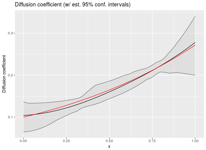
Since it’s so easy to get predictive things out of this approximation, you have a ton of flexibility about using this in weird models. Here I fit a spatially varying diffusion coefficient in a simple PDE IVP (Stan model: https://github.com/bbbales2/gp/blob/master/models/diffusion_gp.stan – if anyone wants the R to run this let me know).
Equation is dc/dt = d(D(x) dc/dx)/dx
With initial conditions: c(0, x) = 0
And Dirichlet boundaries: c(t, -0.5) = c(t, 0.5) = 1)
I used method of lines discretization at like ~10 points on the x axis. Only the data at the final time is used. Grey areas are 95% confidence intervals, red line is truth used to generate the data, dark line is the mean of the posterior:

Or you can estimate a concentration varying diffusion coefficient (dc/dt = d(D(c) dc/dx)/dx, and this uses 20 points on the x-axis if I recall correctly https://github.com/bbbales2/gp/blob/master/models/diffusion_state_gp.stan):
Those were both done with simulated data and I chose two conveniently pretty results :D, so caveat emptor if there’s anyone that cares about diffusion constants floating around here.
Anyhow, that’s a big wall of text hopefully it’s useful to someone. I dunno what the actual name for this stuff is. This seems like maybe it’s the fancier version: http://quinonero.net/Publications/lazaro-gredilla10a.pdf
Edits: Added some more plots to explain how error in the approximation comes about and fixed a few issues I noticed.
Edits 2: Fixed a sampling statement. Tnx Arya