Hi, I’m new to Stan and my model can not converge.
Here’s a brief introduction to my model.
I need to estimate the mortality rate for 21 countys in 21 years (1995~2015). Thus the data is one 21x21 matrix for births x and one for deaths y.
So denote underlying mortality rate as Alpha, this is a binomial distribution with y \sim binomial(x, Alpha). And it is obvious that the mortality rate should be quite small, say 96 deaths out of 22626.
For Alpha, I use a bayesian penalized spline regression model. The original model is shown in this picture (cut from the paper I read).

I did a little change to this original model.
-
\Psi in this original model is the log transformation of true mortality rate. Yet I found that when calculating true rate, \exp(\Psi) are not constrained in [0,1]. So I modeled \Psi as the logit transformation of true rate.
-
The original model has different sources of data, and my data is quite simple, so I simplified the data model part to
\delta_c \sim N(0, \nu_c), \nu_c \sim U(1, 10), suggesting that different county has different variation.
Here’s my stan code.
data {
	int TT; // number of years, 21
	int K; // number of splines, 13
	int C; // number of countys, 21
	real I; // between-knot intervals, set to 2.5 years

	int x[C,TT]; // births
	int y[C,TT]; // deaths
	matrix[K,K-2] D_Kc; // transformation of difference matrix
	matrix[TT,K] B; // calculated cubic spline matrix
}
parameters {
	real chi;
	real<lower=0> phi;
	real sigma_lg[C];
	real<lower=0> lambda_0_exp[C];
	vector[C] lambda_1_unit;
	real<lower=0> nu[C];
	matrix[C,K-2] epsilon;
	row_vector[TT] delta[C];
}
transformed parameters {
	real<lower=0> sigma[C];
	real lambda_0[C];
	vector[C] lambda_1;

	row_vector[K] alpha[C]; // spline coefficients

	sigma = exp(sigma_lg);
	lambda_0 = log(lambda_0_exp);
	lambda_1 = lambda_1_unit * I;

	for (c in 1:C){
		for (k in 1:K)
			alpha[c,k] = lambda_0[c] + lambda_1[c] * (k - K * 1.0 / 2) + D_Kc[k] * epsilon[c]';
	}
}
model {
	chi ~ normal(-3, sqrt(10));
	phi ~ uniform(0,5);
	sigma_lg ~ normal(chi, phi);
	lambda_0_exp ~ uniform(1,1000);
	lambda_1_unit ~ uniform(-0.25, 0.2);
	nu ~ uniform(1, 10);

	for (c in 1:C){
		delta[c] ~ normal(0, nu[c]);
		epsilon[c] ~ normal(0, sigma[c]);
		target += binomial_logit_lpmf( y[c] | x[c] , exp(alpha[c] * B' + delta[c]) );
	}
}
generated quantities {
	row_vector<lower=0, upper=1>[TT] Alpha[C]; // estimated true mortality rate

	for (c in 1:C)
		Alpha[c] = inv_logit(alpha[c] * B' + delta[c]);
}
Here’s my R code.
library(bdefdata)
library(demest)
library(dplyr)
library(purrr)
library(tidyr)
library(boot)
library(latticeExtra)
library(rstan)
library(splines)

options(mc.cores = parallel::detectCores())
rstan_options(auto_write = TRUE)

y <- bdefdata::sweden_deaths
x <- bdefdata::sweden_births
C <- dim(x)[1]
TT <- dim(x)[2]
tpower <- function(x, t, p){
  # Truncated p-th power function
  (x - t) ^ p * (x > t)
}
bbase <- function(x, xl, xr, dx, deg){
  # Construct a B-spline basis of degree ’deg’
  knots <- seq(xl - deg * dx, xr + deg * dx, by = dx)
  P <- outer(x, knots, tpower, deg)
  n <- dim(P)[2]
  D <- diff(diag(n), diff = deg + 1) / (gamma(deg + 1) * dx ^ deg)
  B <- (-1) ^ (deg + 1) * P %*% t(D)
  B
}
B <- round(bbase(1995:2015, 1995, 2015, 2.5, 3), 8)

K <- dim(B)[2]
I <- 2.5
D <- matrix(rep(0, (K-2)*K), nrow=K-2)
for (i in 1:K-2){
  for (j in 1:K){
    if (i == j | j == i + 2) D[i,j] = 1
    if (j == i + 1) D[i,j] = -2
  }
}
D_Kc <- t(D) %*% solve(D %*% t(D))
d <- list(C=C,
          TT=TT,
          K=K,
          I=I,
          x=x,
          y=y,
          D_Kc=D_Kc,
          B=B)

set.seed(12)
initf <- function(chain_id){
  list(lambda_0_exp = runif(C, 1, 1000),
       lambda_1_unit = runif(C, -0.25, 0.2),
       nu = runif(C, 1, 10),
       epsilon = matrix(rnorm(C*(K-2), 0, 1), nrow=C)
       )
}

n_chains <- 6
a <- lapply(1:n_chains, function(id) initf(chain_id = id))
f <- stan(file = 'mr.stan', data = d, chains = n_chains,
             iter = 50000, warmup = 10000, thin = 10,
             control = list(adapt_delta = 0.9),
             init = a)
And the 6 chains do not converge. Warning message suggests “divergent transitions after warmup”, which is almost all of them.
Here’s the traceplot of several Alpha.

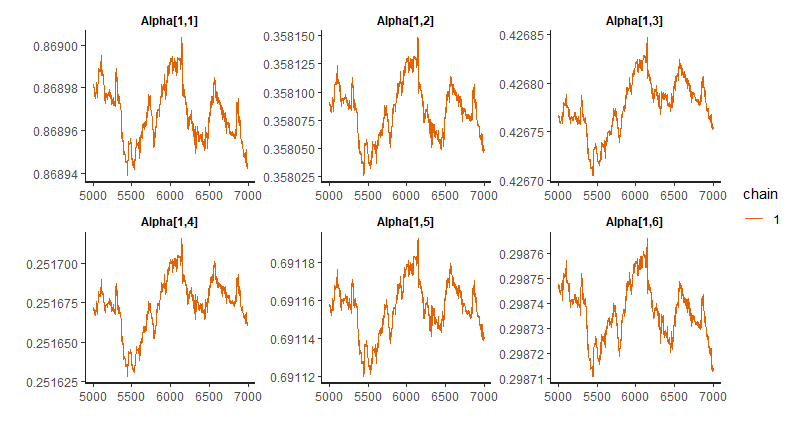
Here’s another traceplot of another run with only one chain.
> sessionInfo()
R version 3.5.3 (2019-03-11)
Platform: x86_64-w64-mingw32/x64 (64-bit)
Running under: Windows 10 x64 (build 18362)

Matrix products: default

locale:
[1] LC_COLLATE=Chinese (Simplified)_China.936
[2] LC_CTYPE=Chinese (Simplified)_China.936
[3] LC_MONETARY=Chinese (Simplified)_China.936
[4] LC_NUMERIC=C
[5] LC_TIME=Chinese (Simplified)_China.936

attached base packages:
[1] splines   stats     graphics  grDevices utils     datasets  methods
[8] base

other attached packages:
 [1] rstan_2.19.3        ggplot2_3.2.1       StanHeaders_2.19.0
 [4] latticeExtra_0.6-28 RColorBrewer_1.1-2  lattice_0.20-38
 [7] boot_1.3-23         tidyr_1.0.0         purrr_0.3.2
[10] dplyr_0.8.3         demest_0.0.0.202    dembase_0.0.0.108
[13] bdefdata_0.0.0.9002
I really need some suggestions. And if there’s naive mistakes in my code, please point them out. Thanks for your time : )

