Hi,
I set up a first-order Poisson Auto-regressive model PAR(1) and tested it on simulated data. During iterating, I hit an example where I get E-BFMI<0.2, but no other warnings, which @betanalpha may be interested in academically.

I do get a compile-time warning, but I thought (perhaps wrongly?) it is okay because the parameters are combined in a linear fashion.
Here is the code, which includes generating the test data:
import numpy as np
import matplotlib.pyplot as plt
import scipy.stats
from numpy import log, pi, cos, exp
import sys

np.random.seed(1)

N = 1000

W = np.random.normal(0, 1, size=N)

T = 1.
dt = T / N
# correlation: set to < 1, otherwise not stationary!
tau = 0.01
phi = exp(-1. / (tau / dt))
#phi = 0.999
print('AR phi:', phi)
print('decay time scale:', tau, 'time interval of sampling:', dt, 'number of steps until decay:', int(tau / dt), 'number of decay timescales sampled:', int(T / tau))
print('OU theta:', - phi * dt)
tau = -1. / log(phi)
gamma = 1. / tau


c = 50.0
sigma = 0.04 * c
y0 = W[0] * sigma + c
y = np.empty(N)
y[0] = y0
t = np.linspace(0, N * T, N)
for i in range(1, N):
	# phi [AR]  corresponds to - theta * dt [OU]
	y[i] = c + phi * (y[i-1] - c) + W[i] * sigma

z = np.random.poisson(y)

plt.figure(figsize=(20, 4))
plt.plot(t, y)
plt.plot(t, z)
plt.xlabel('Time')
plt.ylabel('Value')
plt.savefig('fracar1_t.pdf', bbox_inches='tight')
plt.close()

import stan_utility

model = stan_utility.compile_model_code("""
data {
  int N;
  real dt;
  int<lower=0> z_obs[N];
}
parameters {
  real phi;
  real c;
  real lognoise;
  real<lower=0> y[N];
}
transformed parameters {
  real tau;
  real noise;
  noise = exp(lognoise);
  tau = - dt / log(phi);
}
model {
  phi ~ normal(0, 10) T[0, 100];
  lognoise ~ normal(0, 10);
  for (i in 1:(N-1)) {
     (y[i+1] - c) - phi * (y[i] - c) ~ normal(0, noise);
  }
  z_obs ~ poisson(y);
}
""")

data = dict(N=N, dt=dt, z_obs=z)

results = stan_utility.sample_model(model, data, outprefix="oustanfit", control=dict(max_treedepth=12))

stan_utility.plot_corner(results, outprefix="oustanfit")
And the output:
AR phi: 0.9048374180359595
decay time scale: 0.01 time interval of sampling: 0.001 number of steps until decay: 10 number of decay timescales sampled: 100
OU theta: -0.0009048374180359595
Compiling slimmed Stan code[anon_model_cfe6382326cee97ea72c3e4c8c4d188c]:
  1: data {
  2: int N;
  3: real dt;
  4: int<lower=0> z_obs[N];
  5: }
  6: parameters {
  7: real phi;
  8: real c;
  9: real lognoise;
 10: real<lower=0> y[N];
 11: }
 12: transformed parameters {
 13: real tau;
 14: real noise;
 15: noise = exp(lognoise);
 16: tau = - dt / log(phi);
 17: }
 18: model {
 19: phi ~ normal(0, 10) T[0, 100];
 20: lognoise ~ normal(0, 10);
 21: for (i in 1:(N-1)) {
 22: (y[i+1] - c) - phi * (y[i] - c) ~ normal(0, noise);
 23: }
 24: z_obs ~ poisson(y);
 25: }
DIAGNOSTIC(S) FROM PARSER:
Info:
Left-hand side of sampling statement (~) may contain a non-linear transform of a parameter or local variable.
If it does, you need to include a target += statement with the log absolute determinant of the Jacobian of the transform.
Left-hand-side of sampling statement:
    y[i + 1] - c - phi * y[i] - c ~ normal(...)

INFO:pystan:COMPILING THE C++ CODE FOR MODEL anon_model_cfe6382326cee97ea72c3e4c8c4d188c NOW.

Data
----
  N         : 1000
  dt        : 0.001
  z_obs     : shape (1000,) [30 ... 84]

sampling from model ...
Rejecting initial value:
  Log probability evaluates to log(0), i.e. negative infinity.
  Stan can't start sampling from this initial value.

Gradient evaluation took 0.000184 seconds
1000 transitions using 10 leapfrog steps per transition would take 1.84 seconds.
Adjust your expectations accordingly!


Gradient evaluation took 0.000149 seconds
1000 transitions using 10 leapfrog steps per transition would take 1.49 seconds.
Adjust your expectations accordingly!


Gradient evaluation took 0.000169 seconds
1000 transitions using 10 leapfrog steps per transition would take 1.69 seconds.
Adjust your expectations accordingly!


Rejecting initial value:
  Log probability evaluates to log(0), i.e. negative infinity.
  Stan can't start sampling from this initial value.
Rejecting initial value:
  Log probability evaluates to log(0), i.e. negative infinity.
  Stan can't start sampling from this initial value.
Iteration:    1 / 2000 [  0%]  (Warmup)
Rejecting initial value:
  Log probability evaluates to log(0), i.e. negative infinity.
  Stan can't start sampling from this initial value.
Iteration:    1 / 2000 [  0%]  (Warmup)

Gradient evaluation took 0.000134 seconds
1000 transitions using 10 leapfrog steps per transition would take 1.34 seconds.
Adjust your expectations accordingly!


Iteration:    1 / 2000 [  0%]  (Warmup)
Informational Message: The current Metropolis proposal is about to be rejected because of the following issue:
Exception: normal_lpdf: Scale parameter is 0, but must be > 0!  (in 'unknown file name' at line 22)

If this warning occurs sporadically, such as for highly constrained variable types like covariance matrices, then the sampler is fine,
but if this warning occurs often then your model may be either severely ill-conditioned or misspecified.

Iteration:    1 / 2000 [  0%]  (Warmup)
Iteration:  100 / 2000 [  5%]  (Warmup)
Iteration:  100 / 2000 [  5%]  (Warmup)
Iteration:  100 / 2000 [  5%]  (Warmup)
Iteration:  100 / 2000 [  5%]  (Warmup)
Iteration:  200 / 2000 [ 10%]  (Warmup)
Iteration:  200 / 2000 [ 10%]  (Warmup)
Iteration:  200 / 2000 [ 10%]  (Warmup)
Iteration:  300 / 2000 [ 15%]  (Warmup)
Iteration:  300 / 2000 [ 15%]  (Warmup)
Iteration:  200 / 2000 [ 10%]  (Warmup)
Iteration:  300 / 2000 [ 15%]  (Warmup)
Iteration:  400 / 2000 [ 20%]  (Warmup)
Iteration:  400 / 2000 [ 20%]  (Warmup)
Iteration:  500 / 2000 [ 25%]  (Warmup)
Iteration:  400 / 2000 [ 20%]  (Warmup)
Iteration:  500 / 2000 [ 25%]  (Warmup)
Iteration:  300 / 2000 [ 15%]  (Warmup)
Iteration:  600 / 2000 [ 30%]  (Warmup)
Iteration:  600 / 2000 [ 30%]  (Warmup)
Iteration:  700 / 2000 [ 35%]  (Warmup)
Iteration:  400 / 2000 [ 20%]  (Warmup)
Iteration:  500 / 2000 [ 25%]  (Warmup)
Iteration:  800 / 2000 [ 40%]  (Warmup)
Iteration:  700 / 2000 [ 35%]  (Warmup)
Iteration:  600 / 2000 [ 30%]  (Warmup)
Iteration:  500 / 2000 [ 25%]  (Warmup)
Iteration:  900 / 2000 [ 45%]  (Warmup)
Iteration:  600 / 2000 [ 30%]  (Warmup)
Iteration:  700 / 2000 [ 35%]  (Warmup)
Iteration:  800 / 2000 [ 40%]  (Warmup)
Iteration: 1000 / 2000 [ 50%]  (Warmup)
Iteration: 1001 / 2000 [ 50%]  (Sampling)
Iteration:  700 / 2000 [ 35%]  (Warmup)
Iteration:  800 / 2000 [ 40%]  (Warmup)
Iteration:  900 / 2000 [ 45%]  (Warmup)
Iteration: 1100 / 2000 [ 55%]  (Sampling)
Iteration:  800 / 2000 [ 40%]  (Warmup)
Iteration:  900 / 2000 [ 45%]  (Warmup)
Iteration: 1000 / 2000 [ 50%]  (Warmup)
Iteration: 1001 / 2000 [ 50%]  (Sampling)
Iteration:  900 / 2000 [ 45%]  (Warmup)
Iteration: 1200 / 2000 [ 60%]  (Sampling)
Iteration: 1000 / 2000 [ 50%]  (Warmup)
Iteration: 1001 / 2000 [ 50%]  (Sampling)
Iteration: 1100 / 2000 [ 55%]  (Sampling)
Iteration: 1000 / 2000 [ 50%]  (Warmup)
Iteration: 1001 / 2000 [ 50%]  (Sampling)
Iteration: 1300 / 2000 [ 65%]  (Sampling)
Iteration: 1100 / 2000 [ 55%]  (Sampling)
Iteration: 1200 / 2000 [ 60%]  (Sampling)
Iteration: 1100 / 2000 [ 55%]  (Sampling)
Iteration: 1200 / 2000 [ 60%]  (Sampling)
Iteration: 1400 / 2000 [ 70%]  (Sampling)
Iteration: 1300 / 2000 [ 65%]  (Sampling)
Iteration: 1200 / 2000 [ 60%]  (Sampling)
Iteration: 1500 / 2000 [ 75%]  (Sampling)
Iteration: 1400 / 2000 [ 70%]  (Sampling)
Iteration: 1300 / 2000 [ 65%]  (Sampling)
Iteration: 1500 / 2000 [ 75%]  (Sampling)
Iteration: 1300 / 2000 [ 65%]  (Sampling)
Iteration: 1600 / 2000 [ 80%]  (Sampling)
Iteration: 1400 / 2000 [ 70%]  (Sampling)
Iteration: 1600 / 2000 [ 80%]  (Sampling)
Iteration: 1700 / 2000 [ 85%]  (Sampling)
Iteration: 1500 / 2000 [ 75%]  (Sampling)
Iteration: 1400 / 2000 [ 70%]  (Sampling)
Iteration: 1700 / 2000 [ 85%]  (Sampling)
Iteration: 1800 / 2000 [ 90%]  (Sampling)
Iteration: 1600 / 2000 [ 80%]  (Sampling)
Iteration: 1800 / 2000 [ 90%]  (Sampling)
Iteration: 1500 / 2000 [ 75%]  (Sampling)
Iteration: 1900 / 2000 [ 95%]  (Sampling)
Iteration: 1600 / 2000 [ 80%]  (Sampling)
Iteration: 1700 / 2000 [ 85%]  (Sampling)
Iteration: 1900 / 2000 [ 95%]  (Sampling)
Iteration: 2000 / 2000 [100%]  (Sampling)

 Elapsed Time: 19.0708 seconds (Warm-up)
               11.95 seconds (Sampling)
               31.0208 seconds (Total)

Iteration: 2000 / 2000 [100%]  (Sampling)

 Elapsed Time: 17.0378 seconds (Warm-up)
               14.7212 seconds (Sampling)
               31.759 seconds (Total)

Iteration: 1700 / 2000 [ 85%]  (Sampling)
Iteration: 1800 / 2000 [ 90%]  (Sampling)
Iteration: 1900 / 2000 [ 95%]  (Sampling)
Iteration: 1800 / 2000 [ 90%]  (Sampling)
Iteration: 1900 / 2000 [ 95%]  (Sampling)
Iteration: 2000 / 2000 [100%]  (Sampling)

 Elapsed Time: 20.0447 seconds (Warm-up)
               14.8153 seconds (Sampling)
               34.86 seconds (Total)

Iteration: 2000 / 2000 [100%]  (Sampling)

 Elapsed Time: 21.246 seconds (Warm-up)
               14.8655 seconds (Sampling)
               36.1115 seconds (Total)

WARNING:pystan:Maximum (flat) parameter count (1000) exceeded: skipping diagnostic tests for n_eff and Rhat.
To run all diagnostics call pystan.check_hmc_diagnostics(fit)
WARNING:pystan:Chain 1: E-BFMI = 0.0668
WARNING:pystan:Chain 2: E-BFMI = 0.0811
WARNING:pystan:Chain 3: E-BFMI = 0.0839
WARNING:pystan:Chain 4: E-BFMI = 0.0572
WARNING:pystan:E-BFMI below 0.2 indicates you may need to reparameterize your model
processing results ...
Inference for Stan model: anon_model_cfe6382326cee97ea72c3e4c8c4d188c.
4 chains, each with iter=2000; warmup=1000; thin=1;
post-warmup draws per chain=1000, total post-warmup draws=4000.

           mean se_mean     sd   2.5%    25%    50%    75%  97.5%  n_eff   Rhat
phi        0.89  2.8e-3   0.03   0.83   0.87   0.89   0.91   0.94     99   1.04
c         50.34  8.7e-3   0.58  49.15  49.98  50.36  50.73  51.45   4520    1.0
lognoise   0.55    0.02   0.13   0.29   0.46   0.55   0.65   0.79     49   1.09
y[1]      48.65    0.06   4.02  40.78  45.93   48.6  51.32  56.75   4849    1.0
y[2]      48.63    0.05    3.4  42.26  46.27  48.62  50.87  55.43   4841    1.0
y[3]      48.73    0.05   2.99  43.15  46.68  48.68  50.76  54.76   4245    1.0
y[4]      48.92    0.04   2.77  43.83  47.01  48.84  50.73  54.53   4035    1.0
y[5]      48.77    0.04   2.63  43.67  46.94  48.71   50.5  54.13   3466    1.0
y[6]      48.05    0.04   2.59  42.93  46.28  48.03  49.78  53.29   4257    1.0
y[7]      47.95    0.04   2.49  43.13  46.26  47.91  49.59   53.0   4404    1.0
y[8]      47.43    0.04   2.47  42.56  45.78  47.44  49.07  52.23   4448    1.0
y[9]      46.93    0.04   2.43  42.21  45.26  46.96  48.53  51.69   4360    1.0
y[10]     46.71    0.04    2.4  41.88  45.13  46.69   48.3  51.45   4283    1.0
y[11]     46.36    0.04   2.41  41.63  44.74  46.28  47.98  50.95   4317    1.0
y[12]     46.26    0.04   2.38   41.7  44.66  46.28  47.86  50.87   4600    1.0
y[13]     46.98    0.04   2.41  42.36  45.33  46.96  48.65  51.69   4441    1.0
y[14]     47.25    0.04    2.4  42.59  45.65  47.22  48.84  51.94   4253    1.0
y[15]     47.27    0.03   2.41  42.64  45.59  47.21  48.87   52.2   5278    1.0
y[16]     46.79    0.04   2.41  42.06  45.18   46.8  48.35  51.65   4551    1.0
y[17]     46.68    0.03   2.45  41.83  44.99  46.74  48.36  51.41   5032    1.0
y[18]     47.01    0.04    2.4  42.47  45.36  47.04  48.61   51.8   4606    1.0
y[19]     47.64    0.04   2.38  42.99  46.08   47.6  49.24  52.53   4390    1.0
y[20]     48.28    0.04    2.4  43.61  46.73  48.28  49.83  53.11   4622    1.0
y[21]     48.95    0.04   2.38  44.36  47.39  48.91  50.48   53.7   4140    1.0
y[22]     49.38    0.04   2.38  44.77  47.74  49.38  50.97  54.12   4087    1.0
y[23]     49.75    0.04   2.41   45.1  48.15   49.7  51.31  54.47   4672    1.0
y[24]     50.05    0.04   2.39  45.49  48.45  49.97  51.67  54.72   4663    1.0
y[25]     50.45    0.04   2.39  45.98  48.81   50.4  52.01  55.27   3854    1.0
-- snip, they are all the same --
y[998]    45.93    0.04   2.54   41.0   44.2  45.88  47.68  50.87   4810    1.0
y[999]    45.57    0.04   2.66  40.37  43.74   45.5  47.45  50.81   5131    1.0
y[1000]   45.29    0.04   2.88  39.69  43.34  45.27  47.27  50.87   4731    1.0
tau      9.2e-3  2.8e-4 2.7e-3 5.4e-3 7.4e-3 8.8e-3   0.01   0.02     91   1.04
noise      1.75    0.03   0.23   1.33   1.58   1.74   1.91   2.21     52   1.09
lp__      1.5e5    17.9 123.44  1.5e5  1.5e5  1.5e5  1.5e5  1.5e5     48   1.09

Samples were drawn using NUTS at Fr 05 Mär 2021 11:24:31 .
For each parameter, n_eff is a crude measure of effective sample size,
and Rhat is the potential scale reduction factor on split chains (at
convergence, Rhat=1).
checking results ...
/home/user/.local/lib/python3.8/site-packages/stan_utility-0.1.2-py3.8.egg/stan_utility/utils.py:76: UserWarning: Chain 0: E-BFMI = 0.06682835264021626
  warnings.warn("Chain {}: E-BFMI = {}".format(chain_num, numer / denom))
/home/user/.local/lib/python3.8/site-packages/stan_utility-0.1.2-py3.8.egg/stan_utility/utils.py:76: UserWarning: Chain 1: E-BFMI = 0.08107339340014912
  warnings.warn("Chain {}: E-BFMI = {}".format(chain_num, numer / denom))
/home/user/.local/lib/python3.8/site-packages/stan_utility-0.1.2-py3.8.egg/stan_utility/utils.py:76: UserWarning: Chain 2: E-BFMI = 0.08391842399004969
  warnings.warn("Chain {}: E-BFMI = {}".format(chain_num, numer / denom))
/home/user/.local/lib/python3.8/site-packages/stan_utility-0.1.2-py3.8.egg/stan_utility/utils.py:76: UserWarning: Chain 3: E-BFMI = 0.05720619539756567
  warnings.warn("Chain {}: E-BFMI = {}".format(chain_num, numer / denom))
/home/user/.local/lib/python3.8/site-packages/stan_utility-0.1.2-py3.8.egg/stan_utility/utils.py:84: UserWarning:   E-BFMI below 0.2 indicates you may need to reparameterize your model
You may be glad that I iterated beyond the model written above.
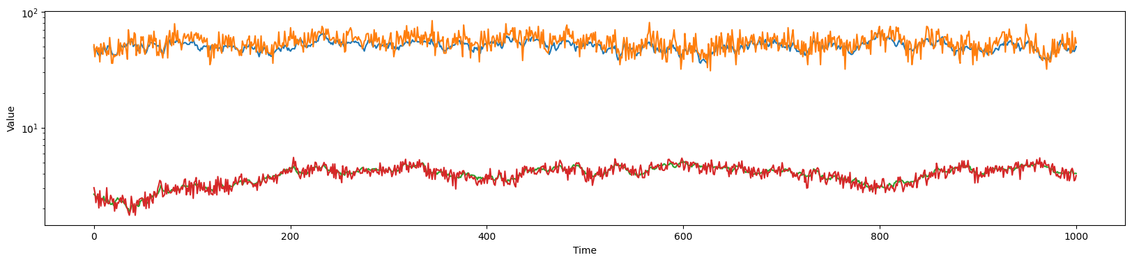
My current setup is the more realistic case (for my problem) of a mixture of two PAR(1) processes, one of which can be observed directly:
import numpy as np
import matplotlib.pyplot as plt
from numpy import log, pi, cos, exp
import sys

np.random.seed(1)

N = int(sys.argv[1])

BW = np.random.normal(0, 1, size=N)
W = np.random.normal(0, 1, size=N)

T = 1.
dt = T / N
# correlation: set to < 1, otherwise not stationary!
tau = 0.01
phi = exp(-1. / (tau / dt))
#phi = 0.999
print('AR phi:', phi)
print('decay time scale:', tau, 'time interval of sampling:', dt, 'number of steps until decay:', int(tau / dt), 'number of decay timescales sampled:', int(T / tau))
print('OU theta:', - phi * dt)

Bc = 100.0
Btau = 0.6
Bsigma = 0.04 * Bc
By0 = BW[0] * Bsigma + Bc
By = np.empty(N)
Bphi = exp(-1. / (Btau / dt))
By[0] = By0
for i in range(1, N):
	# phi [AR]  corresponds to - theta * dt [OU]
	By[i] = Bc + Bphi * (By[i-1] - Bc) + BW[i] * Bsigma

print('phis:', Bphi, phi, Btau, tau)
Bz = np.random.poisson(By)

Barearatio = 1. / 40.0

c = 50.0
sigma = 0.04 * c
y0 = W[0] * sigma + c
y = np.empty(N)
y[0] = y0
t = np.linspace(0, N * T, N)
for i in range(1, N):
	# phi [AR]  corresponds to - theta * dt [OU]
	y[i] = c + phi * (y[i-1] - c) + W[i] * sigma

z = np.random.poisson(y + By * Barearatio)


plt.figure(figsize=(20, 4))
plt.plot(t, y)
plt.plot(t, z)

plt.plot(t, By * (Barearatio if Barearatio > 0 else 1))
plt.plot(t, Bz * (Barearatio if Barearatio > 0 else 1))
plt.yscale('log')
plt.xlabel('Time')
plt.ylabel('Value')
plt.savefig('par1b_t.pdf', bbox_inches='tight')
plt.close()

import stan_utility

model = stan_utility.compile_model_code("""
data {
  int N;
  real dt;
  int<lower=0> z_obs[N];
  int<lower=0> B_obs[N];
  real Barearatio;
}
parameters {
  real logtau;
  real logc;
  real lognoise;
  vector<lower=0>[N] y;

  real logBtau;
  real logBc;
  real logBnoise;
  vector<lower=0>[N] By;
}
transformed parameters {
  real phi;
  real tau;
  real noise;
  real c;

  real Bphi;
  real Btau;
  real Bnoise;
  real Bc;

  tau = exp(logtau);
  c = exp(logc);
  noise = exp(lognoise);
  phi = exp(- 1.0 / (tau / dt));

  Btau = exp(logBtau);
  Bc = exp(logBc);
  Bnoise = exp(logBnoise);
  Bphi = exp(- 1.0 / (Btau / dt));
}
model {
  logBtau ~ normal(-10, 10) T[-100, 0];
  logBc ~ normal(0, 10);
  logBnoise ~ normal(0, 10);
  By[2:N] ~ normal(Bphi * (By[1:(N-1)] - Bc) + Bc, Bc * Bnoise);
  B_obs ~ poisson(By);

  logtau ~ normal(-10, 10) T[-100, 0];
  logc ~ normal(0, 10);
  lognoise ~ normal(0, 10);
  y[2:N] ~ normal(phi * (y[1:(N-1)] - c) + c, c * noise);
  z_obs ~ poisson(y + By * Barearatio);
}
""")

data = dict(N=N, dt=dt, z_obs=z, B_obs=Bz, Barearatio=Barearatio)

results = stan_utility.sample_model(model, data, outprefix="oustanfit", control=dict(adapt_delta=0.99))

stan_utility.plot_corner(results, outprefix="oustanfit")
Here I get no compiler warnings, but a bunch of divergences:
WARNING:pystan:729 of 4000 iterations ended with a divergence (18.2 %).
WARNING:pystan:Try running with adapt_delta larger than 0.99 to remove the divergences.
WARNING:pystan:2604 of 4000 iterations saturated the maximum tree depth of 10 (65.1 %)
WARNING:pystan:Run again with max_treedepth larger than 10 to avoid saturation
WARNING:pystan:Chain 1: E-BFMI = 0.0937
WARNING:pystan:Chain 2: E-BFMI = 0.127
WARNING:pystan:Chain 3: E-BFMI = 0.16
WARNING:pystan:Chain 4: E-BFMI = 0.138
WARNING:pystan:E-BFMI below 0.2 indicates you may need to reparameterize your model
Advice on how to reparametrize is appreciated :-)
I guess one could use a inverse gamma function to derive the By distributions – perhaps they can be marginalised out with some conjugate prior? Not sure. I do want to keep the y-states though, because I want to fourier transform them later – I guess I cannot do that in Stan(?).