How to reparameterize a Gaussian mixture model?

Evgenii · January 24, 2020, 8:48am

Hi, I get two warnings from cmdstan:

38 of 16000 (0.24%) divergent transitions,
E-BFMI = 0.27 is smaller than 0.3.

Is it ok to publish with these results? If not, how can I fix this. Is there a way to reparametrize the model, as the warnings suggest? Thanks!

Code

gaussian_mixture.stan

// Guassian mixture model
data {
  int<lower=1> N;        // number of data points
  real y[N];             // observed values
  real uncertainties[N]; // uncertainties
}
parameters {
  vector[N] y_true;          // true value
  real<lower=0,upper=1> p;   // mixing proportion
  ordered[2] mu;             // locations of mixture components
  real<lower=0> sigma;       // spread of mixture components
}
model {
  sigma ~ normal(0, 0.1);
  mu[1] ~ normal(-1.4, 0.2);
  mu[2] ~ normal(-1.0, 0.2);
  p ~ beta(2, 2);

  for (n in 1:N) {
    target += log_mix(p,
                      normal_lpdf(y_true[n] | mu[1], sigma),
                      normal_lpdf(y_true[n] | mu[2], sigma));
  }

  y ~ normal(y_true, uncertainties);  // Estimate true values
}

gaussian_mixture.py

"""
Run Gaussian mixture model

Usage
------

Instal cmdstanpy and run:

    python gaussian_mixture.py
"""
from cmdstanpy import CmdStanModel


def get_data():
    """Returns data from observations"""
    values =        [-0.99, -1.37, -1.38, -1.51, -1.29, -1.34, -1.50,
                     -0.93, -0.83, -1.46, -1.07, -1.28, -0.73]

    uncertainties = [ 0.12,  0.05,  0.11,  0.18,  0.03,  0.19,  0.18,
                      0.12,  0.19,  0.09,  0.11,  0.16,  0.08]

    return {
        "y": values,
        "uncertainties": uncertainties,
        "N": len(values)
    }


def sample():
    model = CmdStanModel(stan_file="gaussian_mixture.stan")

    fit = model.sample(data=get_data(), seed=2,
                       adapt_delta=0.99, max_treedepth=10,
                       sampling_iters=4000, warmup_iters=2000,
                       chains=4, cores=4,
                       show_progress=True)

    fit.diagnose()
    print(fit.summary())


if __name__ == '__main__':
    sample()
    print('We are done')

Diagnose

Checking sampler transitions treedepth.
Treedepth satisfactory for all transitions.

Checking sampler transitions for divergences.
38 of 16000 (0.24%) transitions ended with a divergence.
These divergent transitions indicate that HMC is not fully able to explore the posterior distribution.
Try increasing adapt delta closer to 1.
If this doesn't remove all divergences, try to reparameterize the model.

Checking E-BFMI - sampler transitions HMC potential energy.
The E-BFMI, 0.27, is below the nominal threshold of 0.3 which suggests that HMC may have trouble exploring the target distribution.
If possible, try to reparameterize the model.

Effective sample size satisfactory.

Split R-hat values satisfactory all parameters.

Processing complete.

Summary

                Mean      MCSE    StdDev         5%       50%       95%     N_Eff   N_Eff/s    R_hat
name                                                                                                
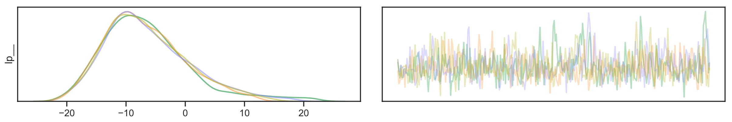
lp__       -6.537390  0.275141  7.408600 -16.793700 -7.586300  7.200930   725.039   32.4301  1.00424
y_true[1]  -0.976441  0.003064  0.126747  -1.237560 -0.952827 -0.807648  1711.500   76.5533  1.00239
y_true[2]  -1.360220  0.000538  0.044592  -1.434220 -1.358910 -1.289390  6866.330  307.1230  1.00008
y_true[3]  -1.354420  0.000832  0.076927  -1.483440 -1.352010 -1.234470  8558.720  382.8210  1.00034
y_true[4]  -1.369540  0.002311  0.110534  -1.549620 -1.365010 -1.206390  2288.200  102.3480  1.00073
y_true[5]  -1.299600  0.000471  0.030118  -1.348380 -1.300000 -1.248750  4082.230  182.5930  1.00059
y_true[6]  -1.312740  0.002470  0.129519  -1.488850 -1.331420 -1.034680  2749.290  122.9720  1.00134
y_true[7]  -1.370810  0.001268  0.103229  -1.546730 -1.363740 -1.215370  6627.500  296.4400  1.00051
y_true[8]  -0.931585  0.001755  0.103812  -1.124750 -0.920968 -0.779502  3500.720  156.5830  1.00013
y_true[9]  -0.938734  0.003833  0.148755  -1.267420 -0.913550 -0.741579  1506.470   67.3827  1.00257
y_true[10] -1.395070  0.001130  0.072108  -1.522230 -1.388680 -1.288920  4070.490  182.0680  1.00074
y_true[11] -1.063860  0.004761  0.149094  -1.322110 -1.034960 -0.856531   980.762   43.8683  1.00256
y_true[12] -1.294110  0.003268  0.128396  -1.458530 -1.318990 -1.013870  1543.310   69.0304  1.00491
y_true[13] -0.819926  0.001357  0.075550  -0.939482 -0.822643 -0.689664  3098.440  138.5900  1.00082
p           0.600030  0.001998  0.146755   0.342263  0.610543  0.824460  5394.000  241.2670  1.00194
mu[1]      -1.344840  0.000956  0.060511  -1.441400 -1.344240 -1.246820  4008.850  179.3110  1.00167
mu[2]      -0.924330  0.001880  0.099102  -1.119760 -0.914959 -0.780432  2778.630  124.2850  1.00200
sigma       0.092938  0.001604  0.054514   0.020375  0.082860  0.197310  1154.410   51.6353  1.00202

Probability trace plot

emiruz · January 24, 2020, 9:18am

Hey Evgenii, would you mind removing your beta prior for p (default is uniform) and reporting back whether the problem gets better or worse? Since you only have few data points, I suspect the priors will effect HMC significantly and prune the parameter space it explores. Others will be able to offer much more insight than me.

Evgenii · January 24, 2020, 9:24am

Unfortunately, I still get 165 of 16000 (1%) divergent transitions, E-BFMI=0.29 warnings after removing the p ~ beta(2, 2); line.

Since you only have few data points

Well spotted! I have another dataset with only 2 times more numbers, for which I don’t get any warnings from Stan.

Thanks for your help, @emiruz!

emiruz · January 24, 2020, 9:31am

No problem. Does that solve your issue or do you need to make it work for the smaller set?

If so, the uniform experiment seems to confirm that it’s something about the prior space. Your mu parameters are very informative given the sample size. Would you mind trying to increase the variance from 0.2 to 1 and reporting the effect? It may enable more of space to be explored.

Evgenii · January 24, 2020, 9:41am

No, unfortunately I still have divergent transitions with the dataset of 13 values from the code above after removing p ~ beta(2, 2); line. What I meant that I have another larger dataset with 27 values, for which this model samples without any warnings.

I still get 138 of 16000 (0.86%) divergent transitions with the following weaker priors:

sigma ~ normal(0, 0.1);
mu[1] ~ normal(-1.4, 1);
mu[2] ~ normal(-1.0, 1);
p ~ beta(2, 2);

stijn · January 24, 2020, 9:59am

Quick guess: Have you checked whether there are strong correlations between the parameters? My guess would be that \mu_1 and \mu_2 could be correlated. If so, you could use the following parameters. \mu_1 and \Delta where \mu_2 = \mu_1 + \Delta with the following prior for \Delta \sim N(0.4, \sqrt{.2^2 +.2^2}).

tiagocc · January 24, 2020, 10:16am

Really interesting stuff! Do you have a reference for this? Thanks

emiruz · January 24, 2020, 10:53am

think the model may have other problems too. y_true has skewed 5% and 95% percentiles but its modeled as normally distributed. do the results change considerably when you alter the priors? if so prior choice becomes important to justify.

Evgenii · January 24, 2020, 12:55pm

Based on this plot, do you think \mu_1 and \mu_2 are correlated?

Thanks, I gave it a go, but still got “112 of 16000 (0.7%) divergent transitions”, and “E-BFMI=0.28” warnings.

See code here.

Evgenii · January 24, 2020, 1:24pm

Well spotted again! :) Yes, I noticed that distributions for some “true” values are not normal at all. For example, on histogram below, you can see that y_true.11 is very uncertain, kind of bimodal.

Isn’t it how it is supposed to work though? You can see from the figure below that the 11th point sits in the middle, so the model is not sure which of the two populations it belongs. It results in two humps on the histogram, so the model “thinks” the “true” value of 11th point is more probable where the population means are.

If I make the prior for mu2 very informative, i.e. change form

mu[2] ~ normal(-1.0, 0.2);

to

mu[2] ~ normal(-1.0, 0.01);

then the peak of posterior distribution for mu2 will be very close to -1. Which is expected, I think. But If I make this prior less informative than now, its posterior distribution remains about the same.

Yes, that’s good point. The priors for mu1, mu2 are not arbitrary, these are stellar sodium abundances that are expected at about -1 \pm 0.5

Evgenii · January 24, 2020, 1:45pm

The model code is based on example from Stan’s documentation. Plus I extended it to account for measurement uncertainties.

Max_Mantei · January 24, 2020, 2:03pm

Maybe a non-centered parameterization of the mixture components works better?

// Guassian mixture model
data {
  int<lower=1> N;        // number of data points
  real y[N];             // observed values
  real uncertainties[N]; // uncertainties
}
parameters {
  real<lower=0,upper=1> p;   // mixing proportion
  ordered[2] mu;             
  real<lower=0> sigma;       // spread of mixture components
  vector[N] z1;
  vector[N] z2;
}
transformed parameters {
  vector[N] y_mix1 = mu[1] + sigma*z1;
  vector[N] y_mix2 = mu[2] + sigma*z2; // I corrected this in an edit!!
}
model {
  sigma ~ normal(0, 0.1);
  mu[1] ~ normal(-1.4, 1);
  mu[2] ~ normal(-1.0, 1);
  p ~ beta(2, 2);
  
  z1 ~ std_normal();
  z2 ~ std_normal();

  for (n in 1:N) {
    target += log_mix(p,
                      normal_lpdf(y[n] | y_mix1[n], uncertainties), // corrected (see edit2 below)
                      normal_lpdf(y[n] | y_mix2[n], uncertainties)); // corrected (see edit2 below)
  }
}
generated quantities{
  vector[N] y_true;
  
  for (n in 1:N)
    y_true[n] = bernoulli_rng(p) == 0 ? y_mix1[n] : y_mix2[n];

}

Can’t make anything of the results though… Do they make sense?

Edit: I corrected something in the code above (see comment in code): the auxillary variable for y_mix2 should be be z2…

Edit2: As pointed out by @Evgenii, y_mix1 and y_mix2 need to be indexed as well in the log_mix call \rightarrow changed to y_mix1[n] and y_mix2[n].

emiruz · January 24, 2020, 2:39pm

It may be my naivity but if y_true are draws from one of two normal posteriors, I guess I’d expect the sampling distribution to be normal for each of them. You could try and double the number of warm up iterations to see if posterior samples look a bit more normal as a result.

Only other things I can think of trying is running the model for generally more iterations and changing the delta_adapt parameter to .99 for example to make HMC take smaller steps.

stijn · January 25, 2020, 1:48am

Not references sorry. It’s the same principle as the uncentered parametrization and one of the tricks people recommend here for autoregressive models. The differences are sometimes more independent than the means and reparametrizarion in terms of differences can help Stan. It did not work in this case unfortunately.

Evgenii · January 25, 2020, 6:15am

Yes, thank you very much! With your reparametrisation, the model runs without any warnings now. This issue is solved! :)

I had to make a little change to your code. I changed from this:

for (n in 1:N) {
    target += log_mix(p,
                      normal_lpdf(y[n] | y_mix1, uncertainties),
                      normal_lpdf(y[n] | y_mix2, uncertainties));
  }

to this (added [n]'s):

for (n in 1:N) {
    target += log_mix(p,
                      normal_lpdf(y[n] | y_mix1[n], uncertainties[n]),
                      normal_lpdf(y[n] | y_mix2[n], uncertainties[n]));
  }

I assumed it was a typo. The way I found the issue is that the code gave unrealistically small spreads of 0.01 for mu1, mu2 and sigma parameters. With the “[n]” fix, the results are the same as with my original code (except that we have no warnings now).

Here is comparison of your original code, with the one with the “[n]” fix, and also the actual “true” values of parameters (I simulated the observations now, just to test the model). The code for this plot is here.

Yes, I think you are right. Anyway, we don’t need y_true values anymore. With @Max_Mantei’s non-centered parameterization everything works. Thanks for your help. 👍

emiruz · January 25, 2020, 7:01am

Hmmm, but I’m guessing that your uncertainties is the standard deviation from the mean and that y is a draw from a normal distribution with a known standard deviation but an unknown mean, isn’t that right? If so, what you did the first time seems correct to me because it takes into account the uncertainty regarding the true value of your data. Will this model not result in an under estimated variance?

Evgenii · January 25, 2020, 7:26am

Yes.

Ok, I won’t pretend I completely understand what @Max_Mantei’s model is doing. :) But I tested it with multiple simulated data sets of different sizes and compared the results. The new model produces posterior distributions that are almost identical to my original model. We compare “Original” (orange) with “Reparametrized fixed” (blue) on this plot, and they are the same:

The new model samples about 6 times slower than my original one, however. But that’s not a problem, I can wait one minute.

emiruz · January 25, 2020, 7:45am

If I’m not mistaken, by eye it looks like the original has a higher variance at every data point. I suppose it’s down to does it fit your use case and whether the extra variance is important. It’s worth trying to run your original model for more iterations and increasing adapt_delta to .99, which I think is the advise the warnings tend to give so you’ve probably already done it.

Evgenii · January 25, 2020, 7:55am

That’s good point. In order to check that, I’ve made a test by simulating observations that have 5x larger measurement uncertainties, and ran the models. The original and @Max_Mantei’s model appear identical again. You can see that the error bars (68% and 95% HPDIs) for the orange and blue markers are the same. Interestingly, we can also see that the green model (previous @Max_Mantei’s model with a typo) does not agree with simulated ‘true’ values for mu1 and mu2. So it’s good to test models haha.

Thanks for the advice. I’ve tried adapt_delta=.99 but it did not help wth my original model unfortunately.

Max_Mantei · January 25, 2020, 12:57pm

Good catch! Yes, this is what I meant to write. Glad to hear that the results makes sense after your correction! :)

Nothing special, its just using the fact that

\begin{aligned} y& \sim N(\mu,\sigma) \\ \leftrightarrow y& = \mu + \sigma*z \text{, with } z \sim N(0,1) \end{aligned}

and N(0,1) is usually nicer for Stan.

You could kind of see it in the plot that you posted earlier (where you assessed the correlation between \mu_1 and \mu_2). If you look at the last row, the spread of \sigma w.r.t. \mu_1 and \mu_2 has as slight funnel shape. That was even a bit more visible when you plotted it with the dots. This shows that there is a geometry in the posterior parameter space that is hard for the sampler to get to. Non-centered parameterization helps to alleviate that problem by changing the the posterior geometry with help of an auxiliary variable (z in the equation above). I’m always a bit sloppy with terms, but I hope that this makes sense. There are a few chapters in the user manual which discuss reparameterizations. This is the one that’s relevant for this discussion.

Cheers!
Max

EDIT: Just to add to this point

…if the geometry is the culprit usually no amount of adapt_delta or iteration is going to save you. This usually only works for “small” problems.

Topic		Replies	Views
Trouble with Gaussian Mixture Model Modeling	10	4098	December 7, 2018
Bayesian Mixture Model Modeling pystan , rstan , fitting-issues , stan , mixture	2	571	December 29, 2022
Efficiency and failed initialization for Gaussian mixture model Modeling	2	482	November 1, 2018
Help reparameterize GP model to remove divergent transitions Modeling rstan , techniques , fitting-issues , performance	33	1769	February 22, 2022
Error Running Sampler for Gaussian mixture model - Help Needed Modeling fitting-issues	2	355	August 28, 2019