Thanks Max, I hadn’t realised that your reformulation was equivalent (but it is clearly) so I learned something useful too!
2 Likes
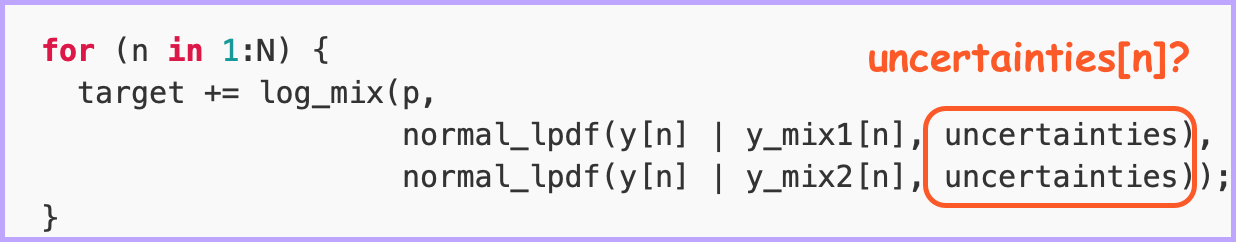
No problem, do we also need uncertainties[n] instead of uncertainties, in the loop? This is what I used.
1 Like
That’s correct, yes. Man I feel a bit stupid. Sorry, I answered way too quickly. With everything indexed correctly, you probably have to up to number of iterations and the adapt_delta. Luckily, you don’t have a huge data set, so that should not be a big problem. I got zero divergent transitions with iter = 8000 and adapt_delta = 0.999, but I didn’t test that much.
1 Like
I think log_mix is vectorized, so you could avoid the loop and do
target += log_mix(p,
                  normal_lpdf(y | y_mix1, uncertainties),
                  normal_lpdf(y | y_mix2, uncertainties))
If this compiles, it’s worth double-checking that you get the same results.
EDIT: my suggestion here implies a different model, find posts below that explain the difference.
I think the vectorized version would imply a different model. At least this is my understanding of the users guide on finite mixture models. I could be wrong, though.
1 Like
Perhaps you are right, thanks for pointing this out!
I know that @andrjohns vectorized logmix (see https://github.com/stan-dev/stan/pull/2532), but documentation has not been updated (https://github.com/stan-dev/docs/issues/134). I hope he’ll be able to clarify if the alternative I propose is really a different model.
1 Like
Feeling stupid is exactly why I like this forum :-) I feel stupid here regularly but never about the same thing; and I’m addicted to it.
4 Likes
That compiles whether log_mix is vectorized or not because normal_lpdf result is always a scalar. The “vectorized” lpdfs have implicit summation and it’s a totally different model.
2 Likes
Updating the documentation for that completely fell off my radar, I’ll that back to the to-do list!
@nhuurre is right about the vectorisation. This model:
for (n in 1:N) {
target += log_mix(p,
normal_lpdf(y[n] | y_mix1[n], uncertainties[n]),
normal_lpdf(y[n] | y_mix2[n], uncertainties[n]));
}
Implies that each observation (individual) has a probability of belonging to each distribution. On the other hand, this model:
target += log_mix(p,
                  normal_lpdf(y | y_mix1, uncertainties),
                  normal_lpdf(y | y_mix2, uncertainties))
Implies that the entire dataset has a probability of belonging to each distribution. In other words, the first specification mixes at the observation level, whereas the second mixes at the dataset level.
The vectorised log_mix just extends the first specification so that you can easily specify a mixture with more than two components. It would be used like the following:
model{
vector[2] contrib[N]; //N = Number of individuals
...other calcs...
for(n in 1:N) {
contrib[n][1] = normal_lpdf(y[n] | y_mix1[n], uncertainties[n]);
contrib[n][2] = normal_lpdf(y[n] | y_mix2[n], uncertainties[n]);
}
target += log_mix(p, contrib);
...rest of model...
}
But you can use an arbitrary number of components, not just 2.
You’re unlikely to see much of a difference in the two-component case though, since the code would be fairly equivalent to the scalar log_mix
3 Likes
Thanks for the tip, I did not know that. I’ve tested the vectorised version of log_mix function:
target += log_mix(p,
                  normal_lpdf(y | y_mix1, uncertainties),
normal_lpdf(y | y_mix2, uncertainties));
The code is here.
I found that this vectorised model produced very different parameter distributions, as can be seen in the plot below. The “Original” orange marker is my original model from the very first post, the “Reparametrized” green one is the model from @Max_Mantei, the blue triangle uses vectorised log_mix function and the vomit-colored rhombuses are the true simulated parameter values.

In addition, the vectorised version sampled pretty badly, with small number of effective samples (N_Eff) and R_hat is way above 1.00:
| Name | Mean | Std | Mode | + | - | 68CI- | 68CI+ | 95CI- | 95CI+ | N_Eff | R_hat |
|---|---|---|---|---|---|---|---|---|---|---|---|
| p | 0.52 | 0.22 | 0.54 | 0.24 | 0.25 | 0.29 | 0.77 | 0.11 | 0.93 | 11 | 1.12 |
| mu.1 | -1.41 | 0.23 | -1.29 | 0.11 | 0.13 | -1.42 | -1.19 | -1.95 | -1.14 | 5 | 1.34 |
| mu.2 | -0.96 | 0.38 | -1.27 | 0.47 | 0.10 | -1.36 | -0.80 | -1.42 | -0.18 | 5 | 1.35 |
| sigma | 0.18 | 0.04 | 0.17 | 0.04 | 0.04 | 0.14 | 0.21 | 0.11 | 0.26 | 6997 | 1.00 |
The traceplot shows that the chains are not well-mixed:

and the pair plot has angled shapes that I honestly have never seen before lol:

So yeah, as other people have pointed out, the vectorised model is a very different one.
Most importantly, to quote @andrjohns, the vectorised version combined with the fact that normal_lpdf function always returns a scalar…
Sorry @Evgenii for making you try that, I had not realised that my formulation implied a different model! Thanks @nhuurre and @andrjohns for explaining that so well, perhaps it will be valuable to others anyway. I’m going to edit my post to mention that already, so that people won’t use my code wrongly if they don’t read to the end.
1 Like
Update: @avehtari suggested an improvement to the model that makes sampling even better.
1 Like