Comparing two models: single gaussian and a mixture of two gaussians

Evgenii · March 2, 2020, 4:10am

@avehtari, thank you so much. I have changed the model as you suggested and that fixed the problem completely! Model comparison now strongly prefers the two-gaussian model, as it should (I did many other tests with synthetic data as well). WAIC and PSIS numbers are almost identical. Pareto K values are all below 0.5.

The new model also samples much faster, with no Stan warnings and higher effective number of samples, so the new model is a better solution to my divergent transitions question.

I’ve also checked that the fixed model produces distributions of model parameters that are almost identical to those from the previous model. So the old and new models are probably mathematically equivalent.

Here is the fixed versions of the models and the plots.

Model 1: single gaussian

// Single Gaussian population model
data {
  int<lower=1> n;        // Number of data points
  real y[n];             // Observed values
  real uncertainties[n]; // Uncertainties
  real sigma_stdev_prior;// Prior for standard deviation of population spread
}
parameters {
  real mu;               // Population location
  real<lower=0> sigma;   // Population spread
}
model {
  // Set priors
  sigma ~ normal(0, sigma_stdev_prior);
  mu ~ normal(0, 1);

  // Loop through observed values and calculate their probabilities
  // for a Gaussian distribution, accounting for uncertainty of each measurment
  for (i in 1:n) {
    target += normal_lpdf(y[i] | mu, sqrt(sigma^2 + uncertainties[i]^2));
  }
}
generated quantities{
  vector[n] lpd_pointwise;

  for (i in 1:n) {
    lpd_pointwise[i] = normal_lpdf(y[i] | mu, sqrt(sigma^2 + uncertainties[i]^2));
  }
}

Model 1: mixture of two gaussians

// Guassian mixture model
data {
  int<lower=1> n;        // Number of data points
  real y[n];             // Observed values
  real uncertainties[n]; // Uncertainties
  real sigma_stdev_prior;// Prior for standard deviation of population spread
}
parameters {
  real<lower=0,upper=1> r;   // Mixing proportion
  ordered[2] mu;             // Locations of mixture components
  real<lower=0> sigma;       // Spread of mixture components
}
model {
  // Set priors
  sigma ~ normal(0, sigma_stdev_prior);
  mu[1] ~ normal(0, 1);
  mu[2] ~ normal(0, 1);
  r ~ beta(2, 2);

  // Loop through observed values
  // and mix two Gaussian components accounting for uncertainty of each measurment
  for (i in 1:n) {
    target += log_mix(1 - r,
      normal_lpdf(y[i] | mu[1], sqrt(sigma^2 + uncertainties[i]^2)),
      normal_lpdf(y[i] | mu[2], sqrt(sigma^2 + uncertainties[i]^2)));
  }
}
generated quantities{
  vector[n] lpd_pointwise;

  for (i in 1:n) {
    lpd_pointwise[i] = log_mix(1 - r,
      normal_lpdf(y[i] | mu[1], sqrt(sigma^2 + uncertainties[i]^2)),
      normal_lpdf(y[i] | mu[2], sqrt(sigma^2 + uncertainties[i]^2)));
  }
}

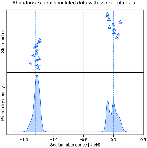
Figure 10: Synthesised observations

Table 1: WAIC output

	WAIC	SE	dWAIC	dSE	pWAIC	Weight
Two populations	-5.06	6.81			3.67	1.00
One population	91.18	4.28	96.24	5.37	3.82	0.00

Table 2: PSIS output

	PSIS	SE	dPSIS	dSE	pPSIS	MaxK	Weight
Two populations	-4.88	6.89			3.76	0.49	1.00
One population	91.20	4.28	96.08	5.43	3.83	0.19	0.00

Topic		Replies	Views
Problematic posterior fit for 2-component Gaussian mixture model Modeling	1	492	August 10, 2019
How to reparameterize a Gaussian mixture model? Modeling	32	3458	March 2, 2020
Incorrect recovery using LOO and WAIC fit indices Modeling loo	10	1038	July 19, 2018
WAIC, AICc and DIC differences in a Bernoulli GLMM in brms vs glmmTMB brms loo	15	3758	October 15, 2018
How to evaluate a Poisson/NB CAR/IAR model General loo	13	2071	February 7, 2019

Comparing two models: single gaussian and a mixture of two gaussians

Model 1: single gaussian

Model 1: mixture of two gaussians

Figure 10: Synthesised observations

Table 1: WAIC output

Table 2: PSIS output

Figure 11: Comparing models with WAIC

Figure 12: Comparing models with PSIS

Figure 13: Pareto K values

Full Code

Comparing two models: single gaussian and a mixture of two gaussians

Model 1: single gaussian

Model 1: mixture of two gaussians

Figure 10: Synthesised observations

Table 1: WAIC output

Table 2: PSIS output

Figure 11: Comparing models with WAIC

Figure 12: Comparing models with PSIS

Figure 13: Pareto K values

Full Code

Related topics