Comparing two models: single gaussian and a mixture of two gaussians

I want to compare two models with WAIC/PSIS, see the code below (the models were reparametrised for better sampling). First model describes a single normally distributed population, and the second model is mixture of two normal populations. In simple language, I want to see if there is one or two populations in my data, according to the models.

Question: what should I use in the “generated quantities” blocks for lpd_pointwise[i] = ... for each model? These are log probability density values for each data point used by WAIC and PSIS.

My brain is too stupid for this :).

Model 1: single gaussian

// Single Gaussian population model
data {
  int<lower=1> n;        // Number of data points
  real y[n];             // Observed values
  real uncertainties[n]; // Uncertainties
  real sigma_stdev_prior;// Prior for standard deviation of population spread
}
parameters {
  real mu;                   // Population location
  real<lower=0> sigma;       // Population spread

  // Normally distributed variable
  vector[n] z1;
}
transformed parameters {
  // Non-centered parametrization
  vector[n] y_mix1 = mu + sigma*z1;
}
model {
  // Set priors
  sigma ~ normal(0, sigma_stdev_prior);
  mu ~ normal(0, 1);

  // Normally distributed variables for non-centered parametrisation
  z1 ~ std_normal();

  // Loop through observed values and calculate their probabilities
  // for a Gaussian distribution, accounting for uncertainty of each measurent
  for (i in 1:n) {
    target += normal_lpdf(y[i] | y_mix1[i], uncertainties[i]);
  }
}
generated quantities{
  vector[n] lpd_pointwise;

  for (i in 1:n) {
    lpd_pointwise[i] = ???
  }
}

Model 1: mixture of two gaussians

// Guassian mixture model
data {
  int<lower=1> n;        // Number of data points
  real y[n];             // Observed values
  real uncertainties[n]; // Uncertainties
  real sigma_stdev_prior;// Prior for standard deviation of population spread
}
parameters {
  real<lower=0,upper=1> r;   // Mixing proportion
  ordered[2] mu;             // Locations of mixture components
  real<lower=0> sigma;       // Spread of mixture components

  // Normally distributed variables
  vector[n] z1;
  vector[n] z2;
}
transformed parameters {
  // Non-centered parametrization
  vector[n] y_mix1 = mu[1] + sigma*z1;
  vector[n] y_mix2 = mu[2] + sigma*z2;
}
model {
  // Set priors
  sigma ~ normal(0, sigma_stdev_prior);
  mu[1] ~ normal(0, 1);
  mu[2] ~ normal(0, 1);
  r ~ beta(2, 2);

  // Normally distributed variables for non-centered parametrisation
  z1 ~ std_normal();
  z2 ~ std_normal();

  // Loop through observed values
  // and mix two Gaussian components accounting for uncertainty
  // of each measurent
  for (i in 1:n) {
    target += log_mix(1 - r,
                      normal_lpdf(y[i] | y_mix1[i], uncertainties[i]),
                      normal_lpdf(y[i] | y_mix2[i], uncertainties[i]));
  }
}
generated quantities{
  vector[n] lpd_pointwise;

  for (i in 1:n) {
    lpd_pointwise[i] = ???
  }
}

What I tried (and failed)

I naively tried copy-pasting code from model block into generated quantities. For single gaussian model:

lpd_pointwise[i] = normal_lpdf(y[i] | y_mix1[i], uncertainties[i]);

and this for the two gaussians:

lpd_pointwise[i] = log_mix(1 - r,
                      normal_lpdf(y[i] | y_mix1[i], uncertainties[i]),
                      normal_lpdf(y[i] | y_mix2[i], uncertainties[i]));

This did not work because in the two-gaussian model the results from normal_lpdf functions are multiplied by (1 - r) and r. And if, for example, r is 0.5 (equal mixture of two gaussians), and a data point is above the peak of the first gaussian, the result of the log_mix function will be about two times smaller than the result from normal_lpdf in the single gaussian model (I plotted posterior distribution on Fig. 4, 5 to help visualise this). Since WAIC are just sums of the log of mean probability density values across sampling iterations (minus effective number of parameters), and the log probability densities for the two-gaussian model are about two times smaller, it follows that the WAIC for the two-gaussian model would also be about two times lower than than that from the single-gaussian model. As a result, the model comparison will always prefer a single-gaussian model, even if the data come clearly from two populations. We are comparing apples with oranges here, I think.

I checked this by synthesising observations with two very distinct gaussian populations shown on Fig.1. Both WAIC and PSIS preferred single gaussian model (see Fig. 2 and 3).

Figure 1: Synthesised observations

Figure 2: Comparing models with WAIC

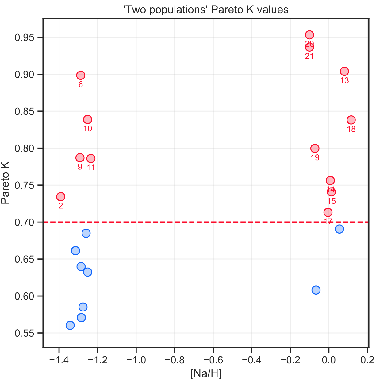
Figure 3: Comparing models with PSIS

Plots of observations and posterior distributions

The thick line on bottom halves of the plots is probability density of observations (not posterior mean). The multiple thin lines are posterior distributions from first 50 iterations. The dashed vertical lines are “true” locations of two synthesised populations.

Figure 4: posterior distributions from one-gaussian model

Figure 5: posterior distributions from two-gaussian model

Full code

The full code to compare the models and make the above plots is located here:

1 Like

Hey again, I went on a similar journey not so long ago. I found this thread very useful: Various approaches to model comparisons

I’ve personally found that model comparison questions require careful formulation. For example, in your case, you may be asking “given that I know the distribution has 1 or more gaussians, how many should I think there are?”. In which case you have just one model, a Gaussian mixture model, and a special interest in the distribution of the parameter governing the number of components.

RE your specific question, for PPC and PSIS/LOO I think you need the log likelihood and samples from your posterior distribution. This is just a matter of copy/pasting your likelihood function from your model and using it’s _rng counterpart for the samples. The arviz quick start guide has a clear Stan example here: https://arviz-devs.github.io/arviz/notebooks/Introduction.html

2 Likes

That’s a good approach, I’ll try that. For now I’m just interested in a single and two-gaussian case.

I did exactly that, described in “What I tried (and failed)” section. It did not work unfortunately. Thanks for the links, they are very useful.

It’s kind of what I mean when I said that model comparison questions require careful formulation. IMHO as always, but I don’t think there’s anything wrong with your likelihood function in the generated quantities. I just think your comparison may be misformulated.

@avehtari has a github page here with lots of examples and recommendations: GitHub - avehtari/modelselection: Tutorial on model assessment, model selection and inference after model selection

IMHO, given that you don’t know which of the two Gaussians (in your mixture case) your observation came from, why would you expect your likelihood to be anything other than the mixture likelihood according to their mixture probabilities? That seems correct to me.

IMO, formulation is the key :-)

1 Like

No it’s not. I would have done exactly what you did.

Can you show the loo diagnostics? That is, the full output from print(your-loo-object)
In your model you have more parameters than observations and I suspect WAIC and PSIS are failing. This is supported also by the fact that WAIC and PSIS values are far from each other. It is possible there is something else also going on there, but without seeing loo diagnostics I don’t start guessing other possibilities.

1 Like

Thanks, that’s very encouraging. :) Here is the output, let me know if you need anything else. You are right, the Pareto K values are really bad (y-axis).

PSIS SE dPSIS dSE pPSIS MaxK Weight
One population -35.89 2.97 19.93 1.06 1.00
Two populations -12.81 5.46 23.07 5.15 16.17 0.95 0.00
WAIC SE dWAIC dSE pWAIC Weight
One population -53.12 2.54 11.31 1.00
Two populations -22.17 4.53 30.95 4.14 11.49 0.00

Worst I ever seen.

Why is y_mix(1|2) a vector and not a scalar? You have now two nested Gaussians, and you could instead use mu and sqrt(sigma^2 + uncertainties[i]^2) which corresponds to integrating analytically over y_mix.

2 Likes

I think @Evgenii is implementing a non centered version and z1 and z2 are vectors and since y_mix(1|2)=mu+sigma*z(1|2) then they have to be as well.

1 Like

@avehtari, thank you so much. I have changed the model as you suggested and that fixed the problem completely! Model comparison now strongly prefers the two-gaussian model, as it should (I did many other tests with synthetic data as well). WAIC and PSIS numbers are almost identical. Pareto K values are all below 0.5.

The new model also samples much faster, with no Stan warnings and higher effective number of samples, so the new model is a better solution to my divergent transitions question.

I’ve also checked that the fixed model produces distributions of model parameters that are almost identical to those from the previous model. So the old and new models are probably mathematically equivalent.

Here is the fixed versions of the models and the plots.

Model 1: single gaussian

// Single Gaussian population model
data {
  int<lower=1> n;        // Number of data points
  real y[n];             // Observed values
  real uncertainties[n]; // Uncertainties
  real sigma_stdev_prior;// Prior for standard deviation of population spread
}
parameters {
  real mu;               // Population location
  real<lower=0> sigma;   // Population spread
}
model {
  // Set priors
  sigma ~ normal(0, sigma_stdev_prior);
  mu ~ normal(0, 1);

  // Loop through observed values and calculate their probabilities
  // for a Gaussian distribution, accounting for uncertainty of each measurment
  for (i in 1:n) {
    target += normal_lpdf(y[i] | mu, sqrt(sigma^2 + uncertainties[i]^2));
  }
}
generated quantities{
  vector[n] lpd_pointwise;

  for (i in 1:n) {
    lpd_pointwise[i] = normal_lpdf(y[i] | mu, sqrt(sigma^2 + uncertainties[i]^2));
  }
}

Model 1: mixture of two gaussians

// Guassian mixture model
data {
  int<lower=1> n;        // Number of data points
  real y[n];             // Observed values
  real uncertainties[n]; // Uncertainties
  real sigma_stdev_prior;// Prior for standard deviation of population spread
}
parameters {
  real<lower=0,upper=1> r;   // Mixing proportion
  ordered[2] mu;             // Locations of mixture components
  real<lower=0> sigma;       // Spread of mixture components
}
model {
  // Set priors
  sigma ~ normal(0, sigma_stdev_prior);
  mu[1] ~ normal(0, 1);
  mu[2] ~ normal(0, 1);
  r ~ beta(2, 2);

  // Loop through observed values
  // and mix two Gaussian components accounting for uncertainty of each measurment
  for (i in 1:n) {
    target += log_mix(1 - r,
      normal_lpdf(y[i] | mu[1], sqrt(sigma^2 + uncertainties[i]^2)),
      normal_lpdf(y[i] | mu[2], sqrt(sigma^2 + uncertainties[i]^2)));
  }
}
generated quantities{
  vector[n] lpd_pointwise;

  for (i in 1:n) {
    lpd_pointwise[i] = log_mix(1 - r,
      normal_lpdf(y[i] | mu[1], sqrt(sigma^2 + uncertainties[i]^2)),
      normal_lpdf(y[i] | mu[2], sqrt(sigma^2 + uncertainties[i]^2)));
  }
}

Figure 10: Synthesised observations

Table 1: WAIC output

WAIC SE dWAIC dSE pWAIC Weight
Two populations -5.06 6.81 3.67 1.00
One population 91.18 4.28 96.24 5.37 3.82 0.00

Table 2: PSIS output

PSIS SE dPSIS dSE pPSIS MaxK Weight
Two populations -4.88 6.89 3.76 0.49 1.00
One population 91.20 4.28 96.08 5.43 3.83 0.19 0.00

Figure 11: Comparing models with WAIC

Figure 12: Comparing models with PSIS

Figure 13: Pareto K values

Full Code

The full code to compare the models and make the above plots is located here:

2 Likes

If I understand correctly then , the solution to this problem was to reduce the number of parameters in the model because PSIS/WAIC require more data than parameters. In this instance that was tantamount to getting rid of the non centred stuff from a previous thread which added vectors z1 and z2.

1 Like

PSIS/WAIC do not require more data than parameters. See, e.g. Figure 1 in Practical Bayesian model evaluation using leave-one-out cross-validation and WAIC where the model has less data than parameters, and it depends on the prior whether the computational approximation in WAIC or PSIS is stable. Furthermore we can divide models with less parameters than data to two categories 1) each parameter in likelihood is influenced by several observations, for example, generalized linear models with more predictors than observations, 2) each parameter in likelihood is influenced just by one observation, for example, “random” effect for each individual. In 1) removing one observation is not removing all the information from the data and that one observation is not necessarily highly influential, in 2) removing one observation removes all information from the data and only the prior matters and then that one observation is likely to be very influential for the corresponding parameter. The example in this thread had case 2 and weak prior on “random” effects.

It’s different whether we reduce by fixing some parameters to fixed values (e.g. 0) or whether we integrate analytically over the parameters. When we integrate over some parameters analytically, the mode doesn’t change and we can still recover the posterior for those parameters if needed.

Non-centered part is completely orthogonal to this issue, and there would be exactly the same problem with the centered parameterization. What matters is that the “random” effects (with weak prior) were presented explicitly instead of integrating them out. Analytical integration was possible as both the latent distribution and observation model are Gaussian. If the observation model would be non-Gaussian we could not integrate analytically and we would need to sample the “random” effects, integrate approximately e.g. using Laplace method, or instead of using explicit “random” effects use related over-dispersed observation model.

1 Like

I see ; that’s very clear . Thank you! In this instance the likelihood function includes vectors z(1|2) (the random effects) which are parameters influenced by exactly one observation hence the source of case 2 effect I guess.

I see how in this instance case 2 could be resolved through integration and ultimately why that may be tricky in analytically intractable cases.

Very clear. Thanks again.