NUTS misses U-turns, runs in circles until max_treedepth

[nhuurre]

This is most likely related to the performance regression discussed by @bbbales2 and @betanalpha in the thread on stepsize adaptation tweak but not directly relevant for that thread’s topic.

NUTS is supposed to automatically select the optimal integration time for HMC and because that should only depend on the geometry of the model I would expect that the number of leapfrog steps NUTS uses for a given model is inversely proportional to the stepsize. That is an overly simplistic argument but even so I was quite surprised by the results of some simulations.

All fits here were done using PyStan 2.19.

The model I tested is a five dimensional vector whose all components have IID standard normal distribution. To keep things simple I used the unit_e metric (which is optimal for standard normal anyway), no warmup, four chains, run for 1000 iterations per chain. Here’s the results of fitting it with 100 different stepsizes:

No divergent transitions occurred during the runs. Even to the right of the vertical red line (where the integrator is theoretically unstable) NUTS criterion cut off the trajectories before they were diagnosed as divergent.

The top graph shows the effective sample sizes for lp__ and the five components of the vector x and grey line is the nominal sample size of 4000. The middle graph shows the average accept_stat__ over the iterations and the bottom graph shows the average n_leapfrog__. Note the logarithmic scale, those spikes are huge.

The problem can be present during warmup even if adaptation eventually finds a stepsize with stable treedepth. Here’s a 500 iteration warmup run for a model of 400 IID standard normals. All control parameters except warmup duration are left to their default values.

When we plot the n_leapfrog__ of each iteration against its stepsize a pattern emerges and it corroborates what can be seen in the first graph.

The vertical grey line is where stepsize freezes after adaptation. Luckily it is in a region of stable treedepth and the model fitting proceeds smoothly with 15 leapfrog steps per posterior draw. Models with 100 to 300 parameters aren’t always as lucky.

Anyway, it seems that whenever the sampler needs to change the treedepth it must visit maximum treedepth first. Let’s think about why that happens.

The sampler builds a trajectory as a binary tree, repeatedly concatenating subtrees until it finds a tree that makes a U-turn. Since we’re sampling from a standard normal distribution the final trajectory will typically look something like three quarters of a circle/ellipse around the origin.

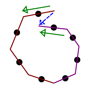
As the stepsize decreases, integration time shrinks proportionally until the trajectory becomes shorter than a semicircle so that it doesn’t quite make a U-turn anymore and the sampler needs to double the number of steps. But two 180 degree U-turns add up to a full 360 degree turn which looks a lot like no turn at all. Therefore at the precise stepsize where treedepth should increase by one, U-turns become invisible and NUTS does not stop until it hits max_treedepth. When stepsize is decreased further the circular trajectory shortens enough to clearly be a steep U-turn and NUTS stabilizes at a new treedepth. This explains what we see in the graphs above.

But hold on, isn’t that impossible? Each subtree is slightly less than a U-turn so their concatenation must be slightly less than a full circle, and that looks like a backward step which the NUTS criterion will detect and stop at. Now, that would indeed be the case if the first point of the second subtree were also the last point on the first subtree but there is in fact one leapfrog step between them. That additional kink in the middle allows two almost-semicircles to overshoot a full circle and avoid termination by NUTS.

A simple fix might be to check the U-turn condition not just at the ends but also in the middle of the new tree. This can be done by changing compute_criterion() in base_nuts.hpp to

      virtual bool compute_criterion(Eigen::VectorXd& p_sharp_minus,
                                     Eigen::VectorXd& p_sharp_middle,
                                     Eigen::VectorXd& p_sharp_plus,
                                     Eigen::VectorXd& rho) {
        return    p_sharp_plus.dot(rho) > 0
               && p_sharp_middle.dot(rho) > 0
               && p_sharp_minus.dot(rho) > 0;
      }

Here p_sharp_middle is the sum of p_sharp at the end of the left subtree and at the start of the right subtree.

Here’s the first graph again after but now using the modified NUTS criterion.

[bbbales2]

@nhuurre

Here’s the first graph again after but now using the modified NUTS criterion.

Hahaha, damnit, I fully planned to keep myself employed for a couple months figuring this out but you’ve gone and done it already. This is cool.

What do you think is next for this?

[betanalpha]

@nhuurre

Since we’re sampling from a standard normal distribution the final trajectory will typically look something like three quarters of a circle/ellipse around the origin.

Technically the optimal trajectory, at least for the component means, is half of a level set which would look like half a great circle for the spherical level sets in this unit normal model.

@nhuurre

That additional kink in the middle allows two almost-semicircles to overshoot a full circle and avoid termination by NUTS.

In addition to the discretization you also have to contend with the fact that the numerical trajectories lie not on the exact level sets but rather modified level sets, and this error can also influence the calculation of the termination criterion.

@nhuurre

A simple fix might be to check the U-turn condition not just at the ends but also in the middle of the new tree.

The complication with tweaks like these is that they require storing many more intermediate states, which then increases the computational burden. The reason for those crude doublings that can have trouble finding the termination point is that they require only a logarithmic number a checks and a logarithmic number of states to be in memory at any given time.

One can also conducer additive expansions where you just add one state at at time, but this requires keeping all states in memory and a quadratic number of checks! See Section A.4.1 of [1701.02434] A Conceptual Introduction to Hamiltonian Monte Carlo.

In other words there is a challenging trade off between the precision in the integration time determination and the overhead for each trajectory. The current multiplicative expansion need not be optimal, but it was chosen to be the most scalable to higher dimensions.

[nhuurre]

The only additional state I am storing is an extra copy of p_sharp_dummy in both transition() and build_tree(). The algorithm follows same doubling behavior, it just inspects both ends of the two subtrees when checking if the full tree is complete.

[bbbales2]

Is it something like this? Where I’ve drawn lines between the sets of points being checked for U-turns?

I’m still thinking in terms of the original uturn criteria btw. I’ve been too lazy to learn the psharp stuff.

[nhuurre]

(So halfway through drawing this I realize the picture is wrong, it should’ve been drawn entirely in the momentum space where R1+R2=R3 does in fact hold, but I think this still gives you the right idea.)

It looks like this:

Let’s say you have built a tree (going from P1 to P2) and because it is not yet a u-turn (the momenta P1 and P2 are not quite orthogonal to R1) you build a second tree (going from P3 to P4). It is also valid so your whole tree is acceptable.

But do you stop here or continue to the next treedepth?

The U-turn criterion is that you check if the momenta at the ends P1 and P4 are parallel or antiparallel to the average momentum R3. Here they are antiparallel and tell us to stop because the picture would have been too confusing if the ends overlapped. But it is possible to imagine a situation where they do cross and R3 is in the opposite direction to what we see here. Then standard NUTS would continue.

The proposed criterion is to also check if P2+P3 is antiparallel to R, which is acceptable here but would bring us to a stop if the ends were crossed (i.e precisely when standard NUTS does not see the u-turn.)

[betanalpha]

@nhuurre

Here p_sharp_middle is the sum of p_sharp at the end of the left subtree and at the start of the right subtree.

But how are you getting the start of the right subtree? What is the modified build_tree code?

[nhuurre]

@betanalpha

But how are you getting the start of the right subtree?

It’s just p_sharp_dummy. p_sharp_dummy starts its life as the right endpoint of the left subtree but because it’s not normally used it gets reused as the left end of the right subtree. I store a copy of it in between. Build_tree proceeds deterministically so there’s no possibility of confusion. (In my first implementation I forgot that transition() moves nondeterministically and the bug made the trajectories twice as long.)

Here’s the full code.

      bool build_tree(int depth, ps_point& z_propose,
                      Eigen::VectorXd& p_sharp_left,
                      Eigen::VectorXd& p_sharp_right,
                      Eigen::VectorXd& rho,
                      double H0, double sign, int& n_leapfrog,
                      double& log_sum_weight, double& sum_metro_prob,
                      callbacks::logger& logger) {
        // Base case
        if (depth == 0) {
          this->integrator_.evolve(this->z_, this->hamiltonian_,
                                   sign * this->epsilon_,
                                   logger);
          ++n_leapfrog;

          double h = this->hamiltonian_.H(this->z_);
          if (boost::math::isnan(h))
            h = std::numeric_limits<double>::infinity();

          if ((h - H0) > this->max_deltaH_) this->divergent_ = true;

          log_sum_weight = math::log_sum_exp(log_sum_weight, H0 - h);

          if (H0 - h > 0)
            sum_metro_prob += 1;
          else
            sum_metro_prob += std::exp(H0 - h);

          z_propose = this->z_;
          rho += this->z_.p;

          p_sharp_left = this->hamiltonian_.dtau_dp(this->z_);
          p_sharp_right = p_sharp_left;

          return !this->divergent_;
        }
        // General recursion
        // XXX replaces p_sharp_dummy
        Eigen::VectorXd p_sharp_lmiddle(this->z_.p.size());

        // Build the left subtree
        double log_sum_weight_left = -std::numeric_limits<double>::infinity();
        Eigen::VectorXd rho_left = Eigen::VectorXd::Zero(rho.size());

        bool valid_left
          = build_tree(depth - 1, z_propose,
                       p_sharp_left, p_sharp_lmiddle, rho_left,
                       H0, sign, n_leapfrog,
                       log_sum_weight_left, sum_metro_prob,
                       logger);

        if (!valid_left) return false;

        // Build the right subtree
        ps_point z_propose_right(this->z_);

        // XXX p_sharp_dummy switches roles here, make a copy instead
        Eigen::VectorXd p_sharp_rmiddle = p_sharp_lmiddle;

        double log_sum_weight_right = -std::numeric_limits<double>::infinity();
        Eigen::VectorXd rho_right = Eigen::VectorXd::Zero(rho.size());

        bool valid_right
          = build_tree(depth - 1, z_propose_right,
                       p_sharp_rmiddle, p_sharp_right, rho_right,
                       H0, sign, n_leapfrog,
                       log_sum_weight_right, sum_metro_prob,
                       logger);

        if (!valid_right) return false;

        // Multinomial sample from right subtree
        double log_sum_weight_subtree
          = math::log_sum_exp(log_sum_weight_left, log_sum_weight_right);
        log_sum_weight
          = math::log_sum_exp(log_sum_weight, log_sum_weight_subtree);

        if (log_sum_weight_right > log_sum_weight_subtree) {
          z_propose = z_propose_right;
        } else {
          double accept_prob
            = std::exp(log_sum_weight_right - log_sum_weight_subtree);
          if (this->rand_uniform_() < accept_prob)
            z_propose = z_propose_right;
        }

        Eigen::VectorXd rho_subtree = rho_left + rho_right;
        rho += rho_subtree;

        // XXX the new check is here
        if ((p_sharp_lmiddle + p_sharp_rmiddle).dot(rho_subtree) < 0)
          return false;

        return compute_criterion(p_sharp_left, p_sharp_right, rho_subtree);
      }

[nhuurre]

Here’s a better picture

Black dots are the position samples. Red lines are momenta along the trajectory. Green lines are summed momenta over the subtrees. The NUTS criterion says that the tree grows until either end of the green line makes at least 90 degree angle with the red line.

(The labels refer not to the points but to the lines, which are understood as vectors. I didn’t draw the arrowheads because the picture feels already too busy. Compare to the other picture if you’re confused.)

In addition to the NUTS criterion (P1 vs R3 and P4 vs R3) there are four possible comparisons one could make:

1. P2+P3 vs R3. This is the most permissive in that if it triggers then these all will trigger. This is what I implemented.
2. P2 vs R3 and P3 vs R3
3. P2+P3 vs R1 and P2+P3 vs R2
4. P2 vs R2 and P3 vs R1. This is the most strict, it will trigger if any of these triggers. This is also how Ben Bales interpreted it in his picture.

The first two can still miss some U-turns while criteria 3 and 4 guarantee (up to numerical rounding errors) that wraparound U-turns are always seen.

I don’t know which one is the best but I guess my current preference is 3.

[betanalpha]

Your argument is that one subtree might just miss the optimal trajectory, and hence the trajectory will have to double by adding a new subtree and then that expanded trajectory might miss again, inciting something of an infinite loop? I can see the first subtree just missing but I don’t see how the first expansion wouldn’t trigger the termination criterion – the trajectory end points should be contracting towards each other causing the termination condition to pass.

Let’s presume that there is an issue with the first expansion because the check against the ends of the doubled trajectory don’t trigger the termination criterion.

You’re then proposing additional checks beyond those at the boundaries of each subtree, right? For example if we wanted to push just a little bit further then we might check against the left-most state and right-most states in each subtree (left image) or the first state and the average momenta between the ends of two subtrees being merged (right image).

I can see how this would help avoid a doubling (at the cost of more checks and carrying around more than just the subtree end points, at least one more state at each level of the recursion) and is worth exploring.

[nhuurre]

@betanalpha

I can see the first subtree just missing but I don’t see how the first expansion wouldn’t trigger the termination criterion – the trajectory end points should be contracting towards each other causing the termination condition to pass.

The endpoints are contracting towards each other and then overshoot before the condition is checked. Yes, this should be impossible as two less-than-U-turns cannot add up to a more than a full circle. But the one leapfrog jump separating the subtrees allows them to rotate towards each other. Your pictures are misleading because they depict the trajectories as continuous. Look at the last picture I posted above and consider the fact that NUTS validity of the subtrees is consistent with any angle whatsoever between the vectors P2 and P3. Checking if R3 is antiparallel to P1 or P4 is not enough.

[bbbales2]

By P2 + P3 vs. R1, do you mean take one additional leapfrog step? Or do you mean check P2 vs R1 and P3 vs R1?

P2 vs R2 and P3 vs R1 look like the original u-turn condition to me the way I’m reading this.

The thing I was talking about looks like the left image in @betanalpha’s third set of plots.

Thanks everyone for taking the time to draw pictures, btw.

[nhuurre]

@bbbales2

By P2 + P3 vs. R1, do you mean take one additional leapfrog step? Or do you mean check P2 vs R1 and P3 vs R1?

I mean check the vector sum of P2 and P3. This is equivalent to checking both P2 vs R1 and P3 vs R1 but continuing even if one of them is negative as long as their sum is positive.

@bbbales2

P2 vs R2 and P3 vs R1 look like the original u-turn condition to me the way I’m reading this.

The original u-turn condition for the left subtree is P1 vs R1 and P2 vs R1.
The original u-turn condition for the right subtree is P3 vs R2 and P4 vs R2
The original u-turn condition for the full tree is P1 vs R3 and P4 vs R3.

P2 vs R2 and P3 vs R1 are new checks ignored by the original u-turn criterion which implicitly assumes that P2=P3 or “close enough”. That’s true in the limit of vanishing stepsize but when the entire tree is only 16 leapfrog steps it’s way too crude.

@bbbales2

Thanks everyone for taking the time to draw pictures, btw.

Thank you for prompting me to do so. It’s been super helpful for clarifying my own thinking about this.

[betanalpha]

I know continuous picture is an idealization, but I’m trying to get a handle on exactly what pathology might be present to ensure that whatever solution we might consider not only resolves that pathology but also doesn’t have any negative influences, such as premature termination of other trajectories. Your initial investigation is intriguing and worth the follow up but we have to figure it out proper before considering a solution!

Excuse the continued to idealized cartoons, but this is the circumstance you thin might be happening, right?

The gap on the right figure is due to the leapfrog between the two subtrees, which pushes the two subtrees to overlap on the other side of the level set.

Wouldn’t the proper checks then be

In other words check between any two subtrees before merging them?

[nhuurre]

Okay, the arguments in this thread have been more difficult to follow than they should have been and that is entirely my fault. Let’s go over some mistakes I’ve made.

Firstly, I’ve provided both code and a picture but I’ve used different names for the same objects. Here’s a quick reference:
P1 = p_sharp_left
P2 = p_sharp_lmiddle
P3 = p_sharp_rmiddle
P4 = p_sharp_right
R1 = rho_left
R2 = rho_right
R3 = rho_subtree

Next, about that picture… it’s supposed to illustrate the new criterion yet depicts a situation where the criterion is redundant and doesn’t even trigger! That’s not helpful, that’s just confusing. Let’s walk through the sampling process step-by-step.

The idea is to build the tree until you find a u-turn. You build a tree with four leapfrog steps. It looks like this:

There is no u-turn here, so you continue and build a second tree. It looks like this:

(Please ignore the fading last node of the first tree, it is not part of this tree.) There is no u-turn here either, so you merge the trees into single big tree. Now the question is, does the big tree have a u-turn? The No-U-Turn criterion we all know and love assumes the tree looks like this:

and tells you: “If the ends of the tree (green) are moving in the general direction of the momenta summed over the whole tree (blue) then there is no u-turn.”

But the tree looks like this:

The No-U-Turn criterion gives you the wrong answer.

Reading Betancourt’s posts again made me understand how to think about this in terms of continuous trajectories. The trajectory is continuous but segmented into timesteps and the u-turn condition is checked using the midpoints of the segments, not their boundaries. Suppose the speed and stepsize are such that it takes 14.5 timesteps to go around the great circle once. Once a trajectory is 8 segments long it starts to contract and should be stopped. However, the discretization error effectively chops off half a segment from both ends and makes the actual comparison with points only 7 segments apart. These are still expanding and the trajectory is doubled to 16 segments. The discretization error again removes one segment and we are left with 15 segments. But since that’s more than 14.5 it wraps around and the trajectory is expanding once again. No evidence of a u-turn has been seen. My proposed solution has been to check if the motion during the “skipped segment” in the middle of the trajectory is in fact antiparallel to the total motion between the checked endpoints.

Moving on.

When you file a bug report you should always include a short piece of code that demonstrates the issue. Something which can be found nowhere in my posts. Oops.

import pystan
import pystan.diagnostics
model = pystan.StanModel(model_code="""
  data {
    int N;
  } parameters {
    vector[N] x;
  } model {
    x ~ std_normal();
  }""")
fit = model.sampling(data=dict(N=200), chains=20,
                     control=dict(max_treedepth=12),
                     refresh=0, check_hmc_diagnostics=False)
pystan.diagnostics.check_treedepth(fit, verbose=3)

WARNING:pystan:24 of 20000 iterations saturated the maximum tree depth of 12 (0.12 %)
WARNING:pystan:Run again with max_treedepth larger than 12 to avoid saturation

I didn’t include rng seed because Stan doesn’t guarantee reproducibility across machines anyway. While the code doesn’t fail every time it does fail often enough that you should have no problem seeing the treedepth warning. You can make the warning happen almost every time by using the default max_treedepth but I wanted the most dramatic example.
The treedepth at which trajectories circle around for this model is 4 because that is what the chains that didn’t blow up have and also what you get with N=500. Those 24 out of 20,000 transitions apparently managed to do 12-4=8 doublings too many which means looping around the origin at least 128 times without noticing a single problem. This is alarming.

And one more thing. I mentioned four alternative new criteria and said that two of them could still miss some u-turns. That was just a guess. Here’s a proper counterexample, a u-turn that the first criterion says isn’t there. (Intermediate points omitted.)

Here R3 and P2 are both downward and even though P3 goes upward it’s so small it has little effect on the average direction at the point where the subtrees join.
It means (p_sharp_lmiddle + p_sharp_rmiddle).dot(rho_subtree) > 0 and my original proposal would not terminate this trajectory.

Looking at the picture we see that there is no room for P3 to align with R3 without also antialigning with R2 (and violating the u-turn condition on the right subtree). If the lengths of R1 and R2 were reversed we could mirror the image and get the same constraint for P2. So checking if either of p_sharp_lmiddle.dot(rho_subtree) or p_sharp_rmiddle.dot(rho_subtree) is negative is in fact a loophole-free condition, contrary to my guess.

[nhuurre]

@betanalpha

I know continuous picture is an idealization

I know you know. It just irks me when the whole problem is the discretization error but you draw a smooth curve and say it can’t happen. Anyway, now that I get the “segmented curve” approach I mentioned in the post above it doesn’t bother me at all.

@betanalpha

premature termination of other trajectories

This is a serious concern. I fear that S-shaped trajectories are in danger. Figure 2 in the Hoffman and Gelman 2014 NUTS paper is a trajectory zig-zagging down a narrow corridor. I think it survives my proposal but it does make me worried.

@betanalpha

idealized cartoons

What’s your opinion on the “momentum polygon” representation I’ve been using? The momentum vectors are placed end-to-end. Subtree momenta are exact and the u-turn criterion is a straighforward statement about the internal angles. Initially I thought it was also accurate in position space when positions are placed in the center of their respective momenta but since then I’ve gotten myself confused again and don’t know anymore.

@betanalpha

In other words check between any two subtrees before merging them?

Yes, but what test do you propose? You can’t compare the p_sharps directly to each other and even if you could it wouldn’t help. All the cheap checks are of the form p_sharp_*.dot(rho_*) > 0 and any symmetric combination of those should be sufficient.

[bbbales2]

@nhuurre

Yes, this should be impossible as two less-than-U-turns cannot add up to a more than a full circle.

@nhuurre

Suppose the speed and stepsize are such that it takes 14.5 timesteps to go around the great circle once.

I think a discretization argument like this is the way to go, but isn’t it true that because of this you can have two half u-turns and get more than a full uturn?

This is because when we put two uturns together, there’s an extra leapfrog in between them? Is that what you’re saying?

Also, I don’t see a reason to separate the momentums and positions in the pictures.

In a lot of leapfrog integrators you have momentums at half-steps and positions at full steps, but Stan needs positions and momentums at the end of every step. With regards to the U-turn criteria I don’t think we need to be thinking about these half-steps.

A couple of the states in the trajectory disappeared in the fourth image. I thought it might have something to do with this.

[bbbales2]

@betanalpha

such as premature termination of other trajectories

@nhuurre

This is a serious concern.

I’m not so sure. We’re just adding checks that would have also been there in the additive scheme, right?

@nhuurre

Yes, but what test do you propose? You can’t compare the p_sharp s directly to each other and even if

It seems like the problem is that we’re too stiff in the distances between points we’re checking over. So we check between certain points L^1 steps apart, then L^2 steps apart, then L^3 steps apart, etc.

And we want to tactically do some checks of lower length? Especially to avoid these things that double a bunch? @avehtari what’s your take on this?

I think we could fix the immediate problem here with checks like on the left of the third figure here: NUTS misses U-turns, runs in circles until max_treedepth - #10 by betanalpha .

[betanalpha]

@nhuurre

This is a serious concern. I fear that S-shaped trajectories are in danger. Figure 2 in the Hoffman and Gelman 2014 NUTS paper is a trajectory zig-zagging down a narrow corridor. I think it survives my proposal but it does make me worried.

When I get home from this trip I’m going to have to put together a test suite of models to systematically check the performance changes.

@nhuurre

What’s your opinion on the “momentum polygon” representation I’ve been using? The momentum vectors are placed end-to-end. Subtree momenta are exact and the u-turn criterion is a straighforward statement about the internal angles. Initially I thought it was also accurate in position space when positions are placed in the center of their respective momenta but since then I’ve gotten myself confused again and don’t know anymore.

It’s tricky to try to align the momenta spatially because of the half-steps in the leapfrog integrator – the distance between points isn’t aligned with either the final or initial momenta. I haven’t wrapped my head around a deeper geometry meaning. Doesn’t mean that something’s not there, just that I’m exhausted from teaching at the moment.

@nhuurre

Yes, but what test do you propose? You can’t compare the p_sharp s directly to each other and even if you could it wouldn’t help. All the cheap checks are of the form p_sharp_*.dot(rho_*) > 0 and any symmetric combination of those should be sufficient.

My intuition is to stick with something that compares subtree ends points to the rho along that subtree because it makes the necessarily reversibility easier to verify – if the checks aren’t sufficiently symmetric then the sampler will pick up an appreciable bias.

Checking between subtrees being merged may not be of much help unless a u turn just happens to be snuck into that niche. I think the more useful check will be between the first points of the merged subtrees (and by symmetry the last points of the merged subtrees) which would terminate trajectories that just missed the u turn after the last doubling. Visually,

Again, I’ll have to verify on a test suite to provide some proper evidence.

[nhuurre]

@bbbales2

We’re just adding checks that would have also been there in the additive scheme, right?

I don’t know what kind of checks you’re thinking of here or what the additive scheme is. I’ve been badly inconsistent on what I propose because there’s a couple of variants and the first one I tried is probably not the best. So I’ll try to be clear here. Currently in build_tree() there is a vector called p_sharp_dummy which is there only so it can be passed to recursive calls. I propose it is replaced by two variables p_sharp_lmiddle and p_sharp_rmiddle to separate it’s two uses. The last line of build_tree which currently reads

return compute_criterion(p_sharp_left, p_sharp_right, rho_subtree);

is then replaced with

return (compute_criterion(p_sharp_left, p_sharp_right, rho_subtree)
     && compute_criterion(p_sharp_lmiddle, p_sharp_rmiddle, rho_subtree));

This is sufficient to prevent the looping.

In other news, I finally did what I should have done a week ago and just hacked Stan to dump the trajectory to std::cout when it goes bad. Here’s what a pathological trajectory actually looks like:

And some more with a larger stepsize. Orange arrows indicate the momentum at the step and the red arrow in the center is the sum of all momenta.

It is perhaps surprising that the ends do not meet. One must remember that the U-turn criterion in Stan is purely a condition on the momenta; the positions are irrelevant. The trajectory stops if the momentum at either end makes at least 90 degree angle with the sum. In all these the momentum has already looped around even though positions are yet to pass.