Hello. I have a model trying to predict if a perspective customer will convert to an actual customer. Usually, I’d use a decision tree to do this but I want to convert…myself into a bayesian modeler. The problem is there are only 327 conversions out of about 9,000 observations. This leaves me with the warning:
UserWarning: Your data appears to have a single value or no finite values
  warnings.warn("Your data appears to have a single value or no finite values")
Below is what the ppc looks like. Is this a “lack of conversion problem” or is my model the problem?
data {
    int<lower=0> N; // number perspective customers
    int<lower=0, upper=1>  issued_flag[N]; // conversion numbers
    vector[N] n_lmt1;// normalized limit 1
    vector[N] n_pp_lmt; //normalized personal property limit
    vector[N] n_age;//normalized age of insured
    vector[N] n_aoh;//normalized age of home

}

parameters {
    real<lower=0> mu;
    real limit1_beta;
    real pplimit_beta;
    real age_beta;
    real aoh_beta;
}

model {
       mu ~ normal(0,3);
       limit1_beta ~ normal(0,5);
       pplimit_beta ~ normal(0,5);
       age_beta ~ normal(0,5);
       aoh_beta ~ normal(0,5);
       issued_flag ~ bernoulli_logit(mu + n_lmt1*limit1_beta + n_pp_lmt*pplimit_beta + n_age*age_beta + n_aoh*aoh_beta);
}

generated quantities {
      vector[N] eta = mu + n_lmt1*limit1_beta + n_pp_lmt*pplimit_beta + n_age*age_beta + n_aoh*aoh_beta;
  int y_rep[N];
  if (max(eta) > 20) {
    // avoid overflow in poisson_log_rng
    print("max eta too big: ", max(eta));
    for (n in 1:N)
      y_rep[n] = -1;
  } else {
      for (n in 1:N)
        y_rep[n] = bernoulli_rng(eta[n]);
  }
}
I would write the model differently, defining a vector in the model block that takes this
mu + n_lmt1*limit1_beta + n_pp_lmt*pplimit_beta + n_age*age_beta + n_aoh*aoh_beta
and sets it equal to a variable that you insert into the Bernoulli_logit function.
model {

vector[N] a;

for n in 1:N {
a[n] = mu + n_lmt1[n]*limit1_beta + n_pp_lm[n]t*pplimit_beta + n_age[n]*age_beta + n_aoh[n]*aoh_beta
}

limit1_beta ~ normal(0,5);
pplimit_beta ~ normal(0,5);
age_beta ~ normal(0,5);
aoh_beta ~ normal(0,5);

issued_flag ~ bernoulli_logit(a)
If I were a better Stan user I could tell you what your code did, but whatever it did I think it was a little off. If you shared your model output it would be easier to see if your model ran correctly.
My guess here is that there is a problem with the way you are passing your data. In your Stan code, there’s a problem in your generated quantities (see below), but I don’t think it could cause the error you are seeing (what interface are you using?).
In generated quantities, you have y_rep[n] = bernoulli_rng(eta[n]); but eta is on the logit scale and you need to use bernoulli_logit_rng. This will produce warnings like
Chain 1 Exception: bernoulli_rng: Probability parameter is -0.0278299, but must be in the interval [0, 1] (in '/var/folders/j6/dg5l3gl11xb9v8w61w99ngh80000gn/T/RtmpjULs5c/model-27aa267750.stan', line 38, column 8 to column 41)
but it shouldn’t yield the behavior that you’re seeing.
Model output like the summary below?
                   Mean      MCSE   StdDev           5%         50%  \
name
lp__         -6300.00000  0.049000  1.70000 -6300.000000 -6300.00000
mu               0.00023  0.000004  0.00023     0.000014     0.00017
limit1_beta     -0.04200  0.005200  0.20000    -0.370000    -0.03900
pplimit_beta     0.05100  0.005200  0.20000    -0.280000     0.04800
age_beta        -0.00053  0.000360  0.02100    -0.035000    -0.00062
...                  ...       ...      ...          ...         ...
y_rep[9083]      0.00000       NaN  0.00000     0.000000     0.00000
y_rep[9084]      0.00000       NaN  0.00000     0.000000     0.00000
y_rep[9085]      0.00000       NaN  0.00000     0.000000     0.00000
y_rep[9086]      0.00000       NaN  0.00000     0.000000     0.00000

                     95%   N_Eff  N_Eff/s  R_hat
name
lp__         -6300.00000  1200.0      4.9    1.0
mu               0.00068  3100.0     13.0    1.0
limit1_beta      0.29000  1500.0      6.2    1.0
pplimit_beta     0.38000  1500.0      6.2    1.0
age_beta         0.03400  3400.0     14.0    1.0
...                  ...     ...      ...    ...
y_rep[9083]      0.00000     NaN      NaN    NaN
Thank you. Here is the updated model I used:
data {
    int<lower=0> N; // number policy
    int<lower=0, upper=1>  issued_flag[N]; // conversion numbers
    vector[N] n_lmt1;// normalized limit 1
    vector[N] n_pp_lmt; //normalized personal property limit
    vector[N] n_age;//normalized age of insured
    vector[N] n_aoh;//normalized age of home

}

parameters {
    real<lower=0> mu;
    real limit1_beta;
    real pplimit_beta;
    real age_beta;
    real aoh_beta;
}

model {
    limit1_beta ~ normal(0,5);
    pplimit_beta ~ normal(0,5);
    age_beta ~ normal(0,5);
    aoh_beta ~ normal(0,5);

    vector[N] a;
    for (n in 1:N) {
            a[n] = mu + n_lmt1[n]*limit1_beta + n_pp_lmt[n]*pplimit_beta + n_age[n]*age_beta + n_aoh[n]*aoh_beta;
    }

    issued_flag ~ bernoulli_logit(a);
}

generated quantities {
      vector[N] eta = mu + n_lmt1*limit1_beta + n_pp_lmt*pplimit_beta + n_age*age_beta + n_aoh*aoh_beta;
  int y_rep[N];
  if (max(eta) > 20) {
    // avoid overflow in poisson_log_rng
    print("max eta too big: ", max(eta));
    for (n in 1:N)
      y_rep[n] = -1;
  } else {
      for (n in 1:N)
        y_rep[n] = bernoulli_logit_rng(eta[n]);
  }
}
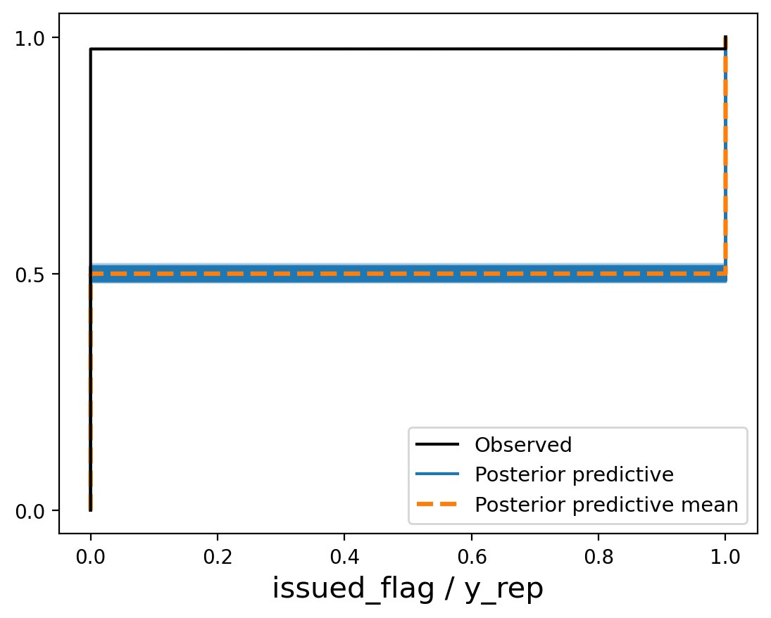
Here is the cumulative ppc output:
Here is the regular ppc output:
Do you think I should be using a different distribution for a convert/not convert target variable?
Since the outcome variable is binary, you are definitely using the right distribution (Bernoulli). It’s very hard to see what’s going on in your graphical posterior predictive plots because the only interesting outcomes are 0 and 1, and these don’t show up adequately on your continuous abscissa. Even from these graphs, however, it’s clear that something is going seriously wrong here.
What’s going wrong is that you’ve declared mu to be greater than zero in the parameters block, but mu is a logit-scale parameter. Given that there are only a few conversions, mu is going to take a negative value. Note that once mu is given a prior consistent with the data, posterior predictive checks based on the total frequency of 1’s and 0’s in the response will no longer be at all sensitive to model misspecification; this is related to the advice (e.g. in @jonah et al’s paper here https://arxiv.org/pdf/1709.01449.pdf) to use statistics of the posterior predictive distribution that are orthogonal to the model parameters.
Ahhh.
I took this model from a previous, poisson model script. I’ve released the floor on mu. This is the result…