A while back I was asking about the simplest way to obtain a posterior predictive check in logistic regression. The ppc_error_binned function in Bayesplot doesn’t seem to work well as I think it requires proportions and not binary 1/0s. Any suggestions would be most appreciated.
Thanks,
David
My modelString is
modelString ="
data {
int <lower=0> n;
vector[n] age;
vector[n] male;
int <lower=0,upper=1> chd[n];
}
parameters {
real alpha;
real beta1;
real beta2;
}
transformed parameters {
real <lower=0> oddsbeta1;
real <lower=0> oddsbeta2;
oddsbeta1 = exp(beta1);
oddsbeta2 = exp(beta2);
}
model {
for (i in 1:n) {
chd[i] ~ bernoulli_logit(alpha + beta1male[i] + beta2age[i]);
}
The code I sent you got a bit messed up in the copying. In any case, the links that were in the previous post about PPCs for logistic regression were not helpful. Here is the code
modelString ="
data {
int <lower=0> n;
vector[n] age;
vector[n] male;
int <lower=0,upper=1> chd[n];
}
parameters {
real alpha;
real beta1;
real beta2;
}
transformed parameters {
real <lower=0> oddsbeta1;
real <lower=0> oddsbeta2;
oddsbeta1 = exp(beta1);
oddsbeta2 = exp(beta2);
}
model {
for (i in 1:n) {
chd[i] ~ bernoulli_logit(alpha + beta1age[i] + beta2male[i]);
}
That did the trick, but I’m still left with the problem of finding the correct way to plot chd against chd_rep. Every plot I try in ppc_ gives very strange figures. chd is coded 1/0, but the model should give the logit of chd and the logit of chd_rep, so a nice simple ppc density or histogram should come out. For example, when I run the following
No worries! This is an area where @jonah would have some good advice. Jonah is there a recommended way to set up the ppc plotting for binary data from a binomal model?
Yeah if you have a binary outcome it can be tricky to think of how to plot it. It’s easier to make plots on the logit scale if you have a binomial outcome with number of trials > 1. But for binary data there are some other options.
Using an rstanarm model as an example:
library(bayesplot)
library(rstanarm)

# switch is 0/1
fit <- stan_glm(switch ~ I(dist/100) + log(arsenic), data = wells, family = binomial)
y <- wells$switch
yrep <- posterior_predict(fit) # draws from the posterior predictive distribution
One thing you can look at is Pr(y = 1) by comparing the proportion of 1s in the data vs the proportions of 1s in the posterior predictive distribution:
ppc_stat(y, yrep, stat = "mean")
You can look at the distribution of other functions too using ppc_stat. The stat argument can be any function that takes in a vector and returns a scalar so, e.g. stat = "sd" would work too.
If you want to look at the distribution of 0s and 1s itself you can use ppc_bars():
ppc_bars(y, yrep)
There are also the ppc_stat_grouped() and ppc_bars_grouped() functions that let you make each of these plots for separate levels of a grouping variable, if that exists in your model.
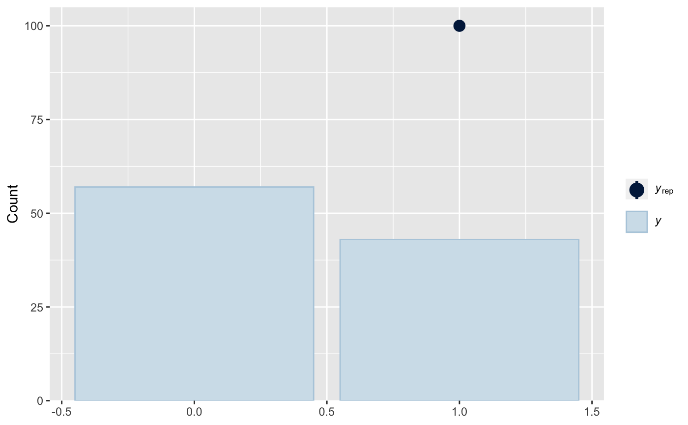
it is telling me that while have about 43% of the sample with heart disease, the model predicts 100% of the sample to have chd. Fairly high number of false positives.
Glad that’s helpful. Yeah it looks like the sample is somewhat balanced but the model is predicting all 1s and no 0s. Presumably the value of
inv_logit(alpha + beta1*age[i] + beta2*male[i])
is coming out to 1 or nearly 1 every time it’s calculated. One thing to consider is that this prior with mean 2 and SD 0.01
is super informative, implying that you pretty much know for sure that beta1 is between 1.97 and 2.03. If that’s true from the prior information you have then that’s fine, but 2 is pretty big on the logit scale so this is probably contributing to the probability being so close to 1.