Divergent transitions

Need some advice on how to reduce or eliminate the divergent transitions with this model. I’m not sure if they even matter as the results are fairly sensible. This is a simple logistic regression model with the outcome whether a health insurance claim was deemed pre-existing or not(approved)PEC_notrauma.txt (34.5 KB) ,and the predictors are age,gender,type of policy and diagnosis.
I can minimise the divergency by cranking up the adapt_delta to 0.999 but this doesn’t seem reasonable.
Tried various priors and not sure how to “re-parameterize” the model.

stanDat <- list(a = as.integer(factor(PEC_notrauma$gender)), 
                b = as.integer(factor(PEC_notrauma$policy)),
                g = as.integer(factor(PEC_notrauma$Diag)),
                y=PEC_notrauma$outcome,
                N = nrow(PEC_notrauma),
                a_N=length(unique(PEC_notrauma$gender)),
                b_N=length(unique(PEC_notrauma$policy)),
                g_N=length(unique(PEC_notrauma$Diag)),
                c=as.matrix(PEC_notrauma$age),#have to store this as a matrix to use this code
                #could be handy if more than one continuous predictor
                c_N=1)

model_string<-
  "data {
int N;
int a_N;                      //  number of categories in gender
int b_N;                      //  number of categories in policy
int g_N;                      // number of categories in diagnosis
int c_N;                      //number of continuous covariates(only 1 here)
int<lower=1, upper=a_N> a[N]; // number applied to gender
int<lower=1, upper=b_N> b[N]; //number applied to policy
int<lower=1,upper=g_N> g[N]; //number applied to diagnosis
matrix[N,c_N] c;                    //observed ages
int<lower=0, upper=1> y[N]; //observed outcome(deemed PEC or approved)
}

parameters {
real intercept;
vector[a_N] a_coeff;
vector[b_N] b_coeff;
vector[g_N] g_coeff;
vector[c_N] c_coeff;
real<lower=0> sigma_a;
real<lower=0> sigma_b;
real<lower=0> sigma_g;
real<lower=0> sigma_c;
real mu_a;
real mu_b;
real mu_g;
real mu_c;
}
transformed parameters {
vector[a_N] normalized_a_coeff;
vector[b_N] normalized_b_coeff;
vector[g_N] normalized_g_coeff;
normalized_a_coeff = a_coeff - a_coeff[1];
normalized_b_coeff = b_coeff - b_coeff[2];
normalized_g_coeff = g_coeff - g_coeff[1];
}
model {
vector[N] p;                  // probabilities
// priors
intercept ~ normal(0,10);//was normal(0,100)
sigma_a ~ normal(0,1); //all the sigmas were cauchy(0,5)
sigma_b ~ normal(0,1);
sigma_g ~ normal(0,1);
sigma_c ~ normal(0,1);
mu_a ~ normal(0,1); // can leave these out and just have 0 as mean of coefficients
mu_b ~ normal(0,1);
mu_g ~ normal(0,1);
mu_c ~ normal(0,1);
// level 1
a_coeff ~ normal(mu_a, sigma_a);
b_coeff ~ normal(mu_b, sigma_b);
g_coeff ~ normal(mu_g, sigma_g);
c_coeff ~ normal(mu_c, sigma_c);
// level 2
for (i in 1:N) {
p[i] = a_coeff[a[i]] + b_coeff[b[i]] + g_coeff[g[i]];
}
y ~ bernoulli_logit(intercept + p + c * c_coeff);//can use poisson_log here;get different parameter estimates
}

generated quantities{
vector[N] y_rep;

for ( n in 1:N ) {

y_rep[n]=bernoulli_logit_rng(intercept + a_coeff[a[n]] + b_coeff[b[n]] + g_coeff[g[n]]+ c[n] * c_coeff);
}
}

"
stan_samples <- stan(model_code = model_string, data = stanDat,warmup=1000,iter=4000,chains=4,
control = list(adapt_delta = 0.95,stepsize=0.01,max_treedepth=15))

I removed one of the diagnostic categories which was a perfect predictor(trauma,all approved).
Regards

Chris

You can non-center all of these:

a_coeff ~ normal(mu_a, sigma_a);
b_coeff ~ normal(mu_b, sigma_b);
g_coeff ~ normal(mu_g, sigma_g);
c_coeff ~ normal(mu_c, sigma_c);

The hows and whys of that are here: https://mc-stan.org/users/documentation/case-studies/divergences_and_bias.html

Non-centering means replacing:

parameters {
  real a;
  real mu;
  real sigma;
}

model {
  a ~ normal(mu, sigma);
}

with

parameters {
  real a_z;
  real mu;
  real sigma;
}

transformed parameters {
  real a = a_z * sigma + mu;
}

model {
  a_z ~ normal(0, 1);
}
3 Likes

Many thanks for your help once again Ben.
I’ll give this a go.
Regards
Chris

So,using

model_string<-
  "data {
int N;
int a_N;                      //  number of categories in gender
int b_N;                      //  number of categories in policy
int g_N;                      // number of categories in diagnosis
int c_N;                      //number of continuous covariates(only 1 here)
int<lower=1, upper=a_N> a[N]; // number applied to gender
int<lower=1, upper=b_N> b[N]; //number applied to policy
int<lower=1,upper=g_N> g[N]; //number applied to diagnosis
matrix[N,c_N] c;                    //observed ages
int<lower=0, upper=1> y[N]; //observed outcome(deemed PEC or approved)
}

parameters {
real intercept;
vector[a_N] a_z;
vector[b_N] b_z;
vector[g_N] g_z;
vector[c_N] c_z;
real<lower=0> sigma_a;
real<lower=0> sigma_b;
real<lower=0> sigma_g;
real<lower=0> sigma_c;
real mu_a;
real mu_b;
real mu_g;
real mu_c;

}

transformed parameters {
vector[a_N] a_coeff = a_z*sigma_a + mu_a;
vector[b_N] b_coeff = b_z*sigma_b + mu_b;
vector[g_N] g_coeff = g_z*sigma_g + mu_g;
vector[c_N] c_coeff = c_z*sigma_c + mu_c;

vector[a_N] normalized_a_coeff;
vector[b_N] normalized_b_coeff;
vector[g_N] normalized_g_coeff;
normalized_a_coeff = a_coeff - a_coeff[1];
normalized_b_coeff = b_coeff - b_coeff[2];
normalized_g_coeff = g_coeff - g_coeff[1];
}
model {
vector[N] p;                  // probabilities
// priors
intercept ~ normal(0,10);//was normal(0,100)
sigma_a ~ normal(0,1); //all the sigmas were cauchy(0,5)
sigma_b ~ normal(0,1);
sigma_g ~ normal(0,1);
sigma_c ~ normal(0,1);
mu_a ~ normal(0,1); // can leave these out and just have 0 as mean of coefficients
mu_b ~ normal(0,1);
mu_g ~ normal(0,1);
mu_c ~ normal(0,1);
// level 1
a_z ~ normal(0,1);
b_z ~ normal(0,1);
g_z ~ normal(0,1);
c_z ~ normal(0,1);
// level 2
for (i in 1:N) {
p[i] = a_coeff[a[i]] + b_coeff[b[i]] + g_coeff[g[i]];
}
y ~ bernoulli_logit(intercept + p + c * c_coeff);//can use poisson_log here;get different parameter estimates
}

generated quantities{
vector[N] y_rep;

for ( n in 1:N ) {

y_rep[n]=bernoulli_logit_rng(intercept + a_coeff[a[n]] + b_coeff[b[n]] + g_coeff[g[n]]+ c[n] * c_coeff);
}
}

"

I still got 246 divergent transitions, although the estimates are sensible.
Maybe I need to fiddle with the priors a bit more.
Do these divergencies matter? It sounds like they do.
Regards
Chris

They do. Even if the predictions/fit look good, divergences basically mean you probably aren’t sampling the thing the equations specify.

I tried this model and with adapt_delta = 0.9 there were divergences, but the main problem was with treedepths.

I noticed in the data that there is only one c. In that case, you don’t want to model that hierarchically cause you’ll just end up with an unidentified parameter. Try not making c hierarchical and up adapt_delta a bit and see where that gets you.

Thanks Ben Using

 "data {
int N;
int a_N;                      //  number of categories in gender
int b_N;                      //  number of categories in policy
int g_N;                      // number of categories in diagnosis
int<lower=1, upper=a_N> a[N]; // number applied to gender
int<lower=1, upper=b_N> b[N]; //number applied to policy
int<lower=1,upper=g_N> g[N]; //number applied to diagnosis
vector[N] c;                    //observed ages
int<lower=0, upper=1> y[N]; //observed outcome(deemed PEC or approved)
}

parameters {
real intercept;
vector[a_N] a_z;
vector[b_N] b_z;
vector[g_N] g_z;
real c_coeff;
real<lower=0> sigma_a;
real<lower=0> sigma_b;
real<lower=0> sigma_g;
real mu_a;
real mu_b;
real mu_g;
}

transformed parameters {
vector[a_N] a_coeff = a_z*sigma_a + mu_a;
vector[b_N] b_coeff = b_z*sigma_b + mu_b;
vector[g_N] g_coeff = g_z*sigma_g + mu_g;

vector[a_N] normalized_a_coeff;
vector[b_N] normalized_b_coeff;
vector[g_N] normalized_g_coeff;

normalized_a_coeff = a_coeff - a_coeff[1];
normalized_b_coeff = b_coeff - b_coeff[2];
normalized_g_coeff = g_coeff - g_coeff[1];
}

model {
vector[N] p;                  // probabilities
// priors
intercept ~ normal(0,10);//was normal(0,100)
c_coeff ~ normal(0,1); //don't model hierarchically as only one coefficient;
sigma_a ~ normal(0,1); //all the sigmas were cauchy(0,5)
sigma_b ~ normal(0,1);
sigma_g ~ normal(0,1);
mu_a ~ normal(0,1); // can leave these out and just have 0 as mean of coefficients
mu_b ~ normal(0,1);
mu_g ~ normal(0,1);

// level 1
a_z ~ normal(0,1);
b_z ~ normal(0,1);
g_z ~ normal(0,1);

// level 2
for (i in 1:N) {
p[i] = a_coeff[a[i]] + b_coeff[b[i]] + g_coeff[g[i]];
}
y ~ bernoulli_logit(intercept + p + c_coeff*c);//can use poisson_log here;get different parameter estimates
}

generated quantities{
vector[N] y_rep;

for ( n in 1:N ) {

y_rep[n]=bernoulli_logit_rng(intercept + a_coeff[a[n]] + b_coeff[b[n]] + g_coeff[g[n]]+ c[n] * c_coeff);
}
}
"
fit <- stan(model_code=model_string,data=stanDat,iter=11000, warmup=1000, chains=1, seed=483892929, refresh=11000,
            control = list(adapt_delta = 0.95))

I got 2 divergent transitions. Is this still too many? Will changing the priors help now?
Regards
Chris

I think you need to change your priors! When I see a wall of normal(0,1) that’s pretty much saying this value might be positive, might be negative, and it’s likely centered around 0. Is that true? If not then getting the priors set right is a great place to start.

Up that adapt_delta a little and they’ll probably go away and you won’t have to sweat about them :D.

Or you can try changing around your priors and stuff like Ara suggests.

1 Like

Thanks Ara.
I think this helped although the parameters are around 0 and can be positive or negative. I got an impression of the priors from running a quick logistic regression model in Stata. Is this cheating?
How else do we get an idea of the priors with many factor levels in the categorical variables?
Anyway the model did converge with your and Ben’s suggestions. The parameter estimates are quite different from the Stata results. I wonder why?
Thanks again.
Regards
Chris

Thanks Ben.
This seemed to work and fiddling with the priors. See my reply to Ada’s post.
Regards
Chris

@Chris_Dalton You are welcome. Can you post the updated model with the new priors? And can you share the stata results? I should have some time this morning to take a look at it.

One other thing. Can you run this with chains = 4 and iter = 2000?

EDIT: Alright I have this up and running with:

fit ← stan(model_code=model_string, data=stanDat, iter=2000, warmup=500, chains=4,
seed=483892929, cores = 6,
control = list(adapt_delta = 0.9999, max_treedepth=14, stepsize=0.01))

I’d check out the pair plots to see if those look reasonable.

library(bayesplot)
mcmc_pairs(as.matrix(fit), pars = c(“c_coeff”,“sigma_a”,“sigma_b”,“sigma_g”,
“mu_a”, “mu_b”,“mu_g”))

Thanks Ara(and Ben) for taking an interest in this small project. I really appreciate it. Just to clarify,I had changed the dataset(dropping one class of the diagnosis factor[trauma]) which I’ll include here.PEC_notrauma.txt (34.5 KB) Using this dataset and this code,I got this to run.I also got it to run using Ara’s Stan calling command above,and the pairs plots look nice and fat so I think this is ok. But I’m still wondering about the Stata output which is different.
Stata_notrauma_output

stan
stanDat <- list(a = as.integer(factor(PEC_notrauma$gender)), 
                b = as.integer(factor(PEC_notrauma$policy)),
                g = as.integer(factor(PEC_notrauma$Diag)),
                y=PEC_notrauma$outcome,
                N = nrow(PEC_notrauma),
                a_N=length(unique(PEC_notrauma$gender)),
                b_N=length(unique(PEC_notrauma$policy)),
                g_N=length(unique(PEC_notrauma$Diag)),
                c=(PEC_notrauma$age))

S<-as.data.frame(stanDat)


model_string<-
  "data {
int N;
int a_N;                      //  number of categories in gender
int b_N;                      //  number of categories in policy
int g_N;                      // number of categories in diagnosis
int<lower=1, upper=a_N> a[N]; // number applied to gender
int<lower=1, upper=b_N> b[N]; //number applied to policy
int<lower=1,upper=g_N> g[N]; //number applied to diagnosis
vector[N] c;                    //observed ages
int<lower=0, upper=1> y[N]; //observed outcome(deemed PEC or approved)
}

parameters {
real intercept;
vector[a_N] a_z;
vector[b_N] b_z;
vector[g_N] g_z;
real c_coeff;
real<lower=0> sigma_a;
real<lower=0> sigma_b;
real<lower=0> sigma_g;
real mu_a;
real mu_b;
real mu_g;
}

transformed parameters {
vector[a_N] a_coeff = a_z*sigma_a + mu_a;
vector[b_N] b_coeff = b_z*sigma_b + mu_b;
vector[g_N] g_coeff = g_z*sigma_g + mu_g;

vector[a_N] normalized_a_coeff;
vector[b_N] normalized_b_coeff;
vector[g_N] normalized_g_coeff;

normalized_a_coeff = a_coeff - a_coeff[1];
normalized_b_coeff = b_coeff - b_coeff[2];
normalized_g_coeff = g_coeff - g_coeff[1];
}

model {
vector[N] p;                  // probabilities
// priors
intercept ~ normal(0,10);//was normal(0,100)
c_coeff ~ normal(0,1); //don't model hierarchically as only one coefficient;
sigma_a ~ normal(0,1); //all the sigmas were cauchy(0,5)
sigma_b ~ normal(0,1);
sigma_g ~ normal(0,1);
mu_a ~ normal(0,2); // can leave these out and just have 0 as mean of coefficients
mu_b ~ normal(0,2);
mu_g ~ normal(0,2);

// level 1
a_z ~ normal(0,3);
b_z ~ normal(0,3);
g_z ~ normal(0,3);

// level 2
for (i in 1:N) {
p[i] = a_coeff[a[i]] + b_coeff[b[i]] + g_coeff[g[i]];
}
y ~ bernoulli_logit(intercept + p + c_coeff*c);//can use poisson_log here;get different parameter estimates
}

generated quantities{
vector[N] y_rep;

for ( n in 1:N ) {

y_rep[n]=bernoulli_logit_rng(intercept + a_coeff[a[n]] + b_coeff[b[n]] + g_coeff[g[n]]+ c[n] * c_coeff);
}
}
"
fit <- stan(model_code=model_string,data=stanDat,iter=11000, warmup=1000, chains=1, seed=483892929, refresh=11000,
            control = list(adapt_delta = 0.99,max_treedepth=15)) #this seems to work

I had loosened up the priors but should I have tightened them up? This seems to be a darker art than tuning your rear derailleur.
Regards
Chris

Thanks Chris. I’ll give this new one a run.

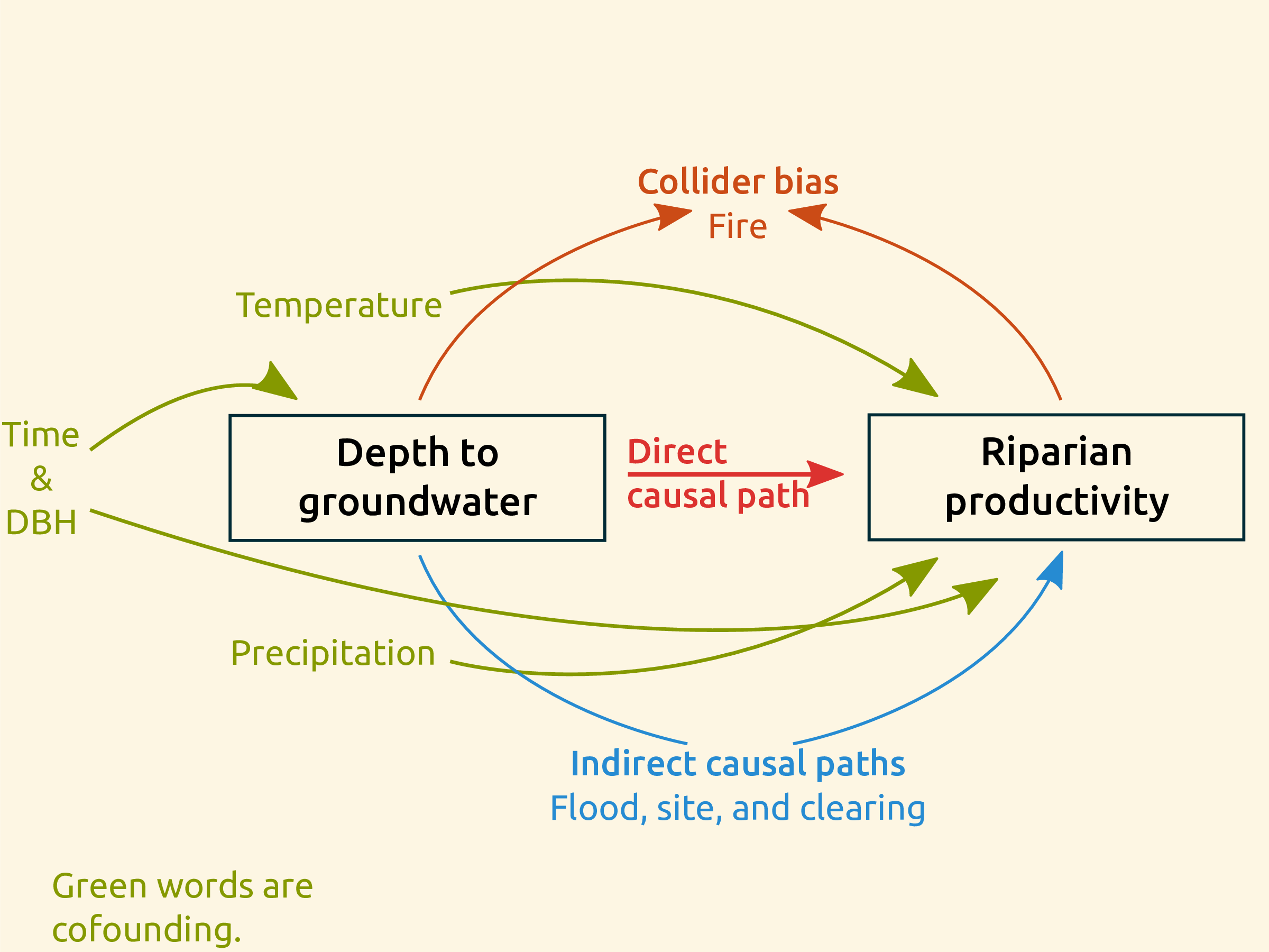
As for priors what I typically do is build out a model like this one
DAG_of_litterfall_model

And for each variable we go through and assign priors based on what we know. For each prior we document how we know this: peer reviewed journal, field notes, panel of experts, and so on. This typically gives decent starting priors.