Hierarchical model 101: Link, categorical without baseline, posterior predictive checks

[cdaube]

Dear brms users,

I feel my questions are more general modeling related than specifically to brms, but since I used brms to fit the model, I thought I should post it here, perhaps also to reflect that I am a beginner with bayesian stats and modeling, and relatively bad at using R, and completely illiterate with stan.

That being said, I was wondering if I could get some opinions on setting up a hierarchical model, or keywords I should use for searching to further inform me. I feel like this post has become quite long and apologise for this. Should you frown on the novel I have written below and have suggestions for a different strategy to get help / progress on my own, before embarking on reading it, they are most welcome!

I want to model correlations, which are the result of many performance evaluations of a “machine-learning” (ml) model I built independently from this brms model. It predicts time series, performances ranging between (pearson correlation) .1 and .4.
I guess that ideally, I would implement this initial ml model already in a bayesian framework, however, I feel that a good hierarchical model for model performances of any generic model would be a nice thing to have and a good way for me to step into hierarchical modeling.
I use a nested-cross-validation approach where I train the ml model on a part of the data, validate it on another and test it on a third, and the associations of data portions to train, validate and test sets are circularly permuted, so that I end up with 6 “outer fold” performances (correlations) for each unit and subunit.

So I have performance evaluations for 24 units, each of them having 2 subunits, all of which I am predicting from various “feature spaces”, i.e. sets of predictors. Ultimately, I am interested to what extent these feature spaces differ in terms of the predictive performance achievable with them, which I want to do with a dummy-coded categorical variable indicating the slope from a baseline feature space to a feature space of interest (i.e. I want to compare the “fixed effects” of feature spaces against each other, for which I am basically relying on the brms hypothesis function, yielding evidence ratios in favour of tested hypotheses of interest like “beta_a > beta_b”).
Additionally, I am including random intercepts for the units, random slopes for the feature spaces for each unit and random slopes for all outer folds (an additional categorical predictor), and interactions between subunits and the feature spaces.

I have various questions:

• how bad is it to use family=“gaussian”? Must I Fisher-Z transform my correlations before entering them into the model? Is there a link function that does this? I constrained the betas with lower and upper boundaries of -2 and +2, reflecting the minimal and maximal values they could take for correlations, however, this is not possible for the intercept (i.e. restricting it between -1 and +1), since " currently, boundaries are only allowed for population level and autocorr parameters", which makes me think the whole idea of setting boundaries is a bad one - do you share this view?
• I read in Gelman’s book that in a bayesian model, I don’t have to use a baseline category for my dummy variables but can instead include variables for all feature spaces instead without running into problems of non-identifiability (p.245 and p.393 from book version of 9. August 2006) – did I misunderstand something here? Or is that really the case?
• when I run this model and do posterior predictive checks, I observe that the yreps have values that are higher than the data:
  
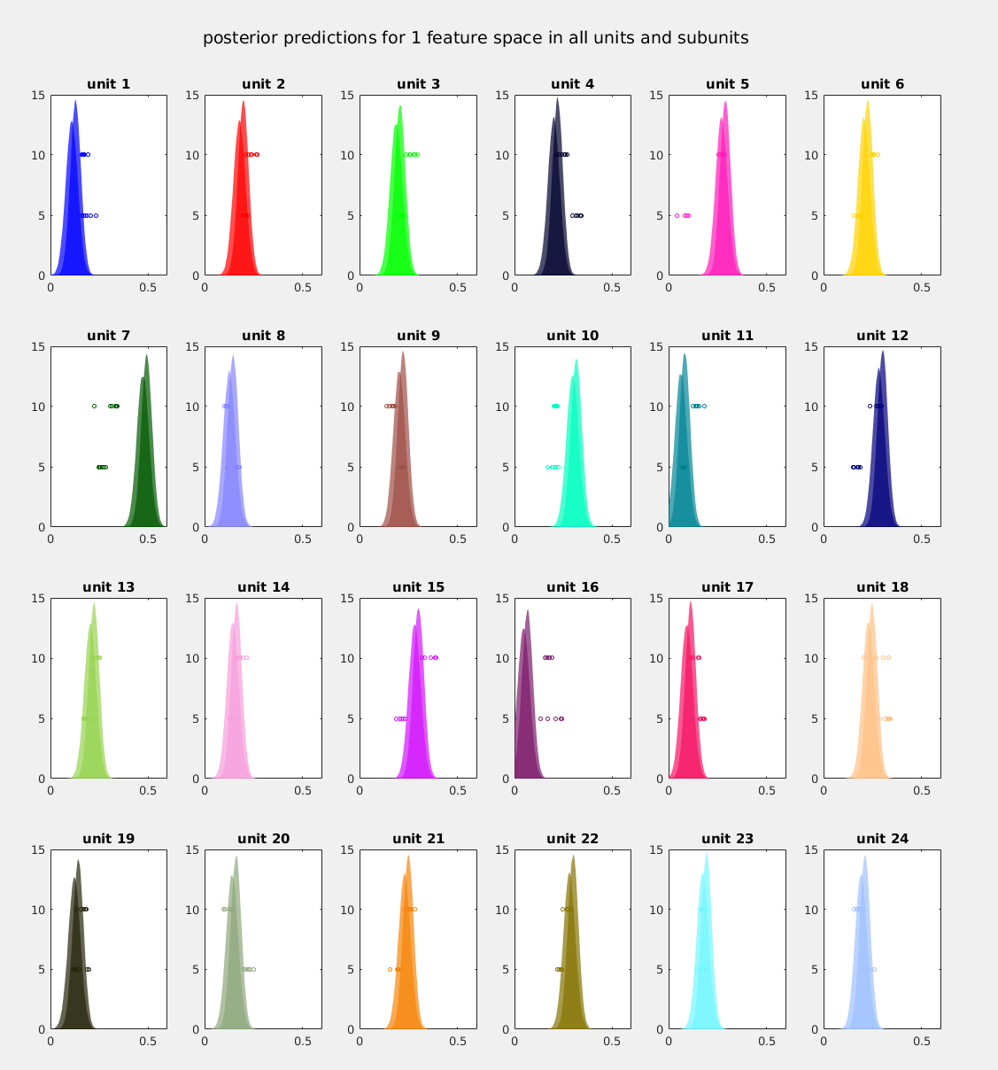
  Specifically, I am referring to the bump we can see at ~.5. I extracted some samples from the yreps and looked at the single units, basically finding that the predictions for one single unit are strongly higher than the observed values:
  
  
  
  In this plot, each actual data point is plotted as a scatter, the y-value being different for the 2 subunits, and the posterior predictive distributions are plotted as ksdensities, one for each subunit in the same plot. It is easy to see that i) many subunits are off from the observed data and ii) unit 7 is highly overestimated, which happens for all feature spaces and consistently across samples from the posterior predictive.
  Is this a degree of disagreement of y and yrep that is unacceptable and points to mistakes in setting up the model? Or is this what people mean when they write “we don’t want to perfectly retrodict the sample”?
• The trained eye will see that this was not done in R, but in matlab instead where I am a lot faster in doing data wrangling like this – I believe there must be a simple way to extract posterior predictive samples corresponding to a given unit / subunit / …? If someone could tell me the keyword I should be looking for in bayesplot, I would be very thankful!
• in terms of the model design, before I read into hierarchical modeling, I had the intuition that I should model the units and subunits as different levels; however, I was discouraged from this by prominent helpers, who said that the 2 subunits are not enough to estimate a variance as necessary for “random effects”; then again, I read in the Gelman book (2006) that he thinks it should be fine, or actually in this case not make much of a difference - I would be interested in any further opinions on this!
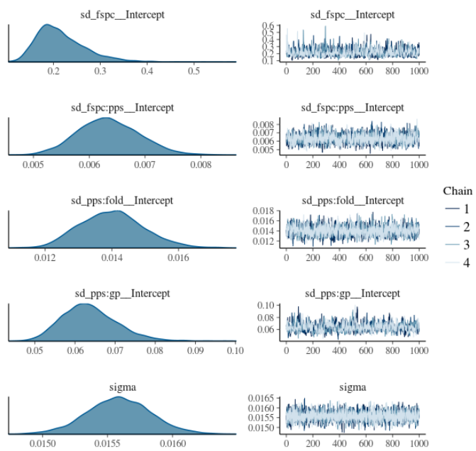
• finally, of course also I am unsure about the priors – the model ran well with uniform priors (-2 – +2 for the intercept, -1 – +1 for the betas), but this seems to be discouraged; additionally, I could imagine that the default sd priors for the random effects might be a bit too broad? Is it a problem to stick to the default LKJ priors for the correlations?

• Operating System: Ubuntu 16.04 LTS
• brms Version: 2.2.0
• model code:
  pps: units
  gp: subunits
  idx_1 – idx_8: dummy variables for feature spaces
  f2 – f6: dummy variables of outer folds
  brmsModel <- brm(r ~ (1|pps) + # random intercept for all levels
  (idx_1-1|pps) + # uncorrelated random slopes for all feature spaces
  (idx_2-1|pps) +
  (idx_3-1|pps) +
  (idx_4-1|pps) +
  (idx_5-1|pps) +
  (idx_6-1|pps) +
  (idx_7-1|pps) +
  (idx_8-1|pps) +
  (f2-1|pps) + # uncorrelated random slopes for folds
  (f3-1|pps) + #
  (f4-1|pps) + #
  (f5-1|pps) + #
  (f6-1|pps) + #
  (gp-1|pps) + # uncorrelated random slope for subunit
  gp*(idx_1 + idx_2 + idx_3 + idx_4 + idx_5 + idx_6 + idx_7 + idx_8 + f2 + f3 + f4 + f5 + f6), # fixed effects
  data = cv8fspc, family = gaussian(),
  cores = 4, iter = 5000, chains = 4, warmup = 1000,
  prior = c(set_prior(“normal(0.1,10)”, class = “Intercept”),
  set_prior(“normal(0.1,10)”, lb = -2, ub = 2, class = “b”)), # ub and lb to reflect boundaries of correlation;
  control = list(adapt_delta = .95, max_treedepth = 15))

Any help would be much appreciated!

[paul.buerkner]

There are a lot of questions in here, so I try to answer some of them.

1. gaussian seems like an ok assumption. Maybe skew_normal would be a little bit better.

2. z-transformation is unlikely to be required for your data since within -0.3 and 0.3 this transformation is almost linear. It may improve things a little bit though.

3. You may fit all categories of a categorical predictor by modeling them with a varying effect term (1|variable).

4. If you don’t want correlations between varying effects to be estimated, you can simply write || instead of |, e.g. (1 + idx_1 + idx_2 || pps).

[cdaube]

Thanks a lot, Paul, this helps a lot!

Regarding 3.: Would it then also be possible to include the random slopes for the categorical predictors with respect to the units, i.e. what I am doing now with the admittedly cumbersome
(idx_1-1|pps)? It doesn’t straightforwardly occur to me how this would be done then. Would that be something like (1|pps/variable)?

[paul.buerkner]

You have to explain your variables to me. What is idx_1, pps and variable?

[cdaube]

Right, sorry:
pps: grouping factor of units (“participants” in this case)
idx_1 – idx_8: binary dummy variables for 8 feature spaces
variable: name of categorical variable created from idx_1 – idx_8 (that’s how I understood your previous post). I would suggest to rename it to fspc (“feature space”) for the sake of clarity in this discussion. Now I have a hunch that your choice of naming it variable was pointing to the flexibility of putting anything there.

So my problem was understanding how to get the random slopes for the effects of each of the dummy variables idx_1 – idx_8 with respect to the grouping factor pps when the “slot” for the grouping variable pps behind the pipe is already occupied by fspc.

Rereading your 2017 arXiv manuscript might have gotten me at least a bit further away from my cargo-cult stats practice. With the initially suggested (1|pps/fspc), I am getting a varying effect for each combination of each level of pps and each level of fspc, which is what I am looking for. But I am not interested in the r_pps[n,Intercept] this would yield. Instead, I want the r_fspc[n,Intercept], so I am switching it to (1|fspc/pps).

I am then tempted to also incorporate the two-leveled subunits gp and the folds by simply using (1 || fspc/pps:gp:folds + gp + folds), where folds would be the outer folds of the cross validation, currently dummy coded as f1 – f6, transformed into one categorical variable, and the + gp + folds would give me additional “main effects” of the subunits gp and the folds, which I am interested in. This however seems to be non-trivial to get to converge. 3 of my 4 chains are done quite quickly, but the last one always takes ages and then has many divergent samples.

[paul.buerkner]

I am sorry, you are loosing me at some point. How did you create fspc from the idx_<n> variables?

If you go for (idx_1 - 1 | pps) + (idx_2 - 1 | pps) + ... your are effectivey fitting a mean parameter for each level of each idx_<n> variable for very person. Is that really what you want?

[cdaube]

Sorry for being unclear.
fspc was created from the idx_<n> variables by transforming matrices of one-hot vectors into integer vectors:

A matrix of [idx_1 idx_2 idx_3 idx_4 idx_5 idx_6 idx_7 idx_8], where each idx<n> is a column vector with 8 rows, i.e.

1 0 0 0 0 0 0 0
0 1 0 0 0 0 0 0 
0 0 1 0 0 0 0 0
...
0 0 0 0 0 0 0 1

would become one column vector of 8 rows, i.e.

1
2
3
...
8

Then of course in the final data frame, there wouldn’t be just 8 rows, but 8(fspc) * 24(pps) * 2(gp) * 6(folds) = 2304 rows.
So fspc is essentially in the same integer-column-vector format as pps, which ranges from 1 to 24.

I suppose there was a typo and you meant

[1] (idx_1 - 1 | pps) + (idx_2 - 1 | pps) + ...

I believed that if combined with “fixed effects” for each level of fspc, i.e.

[2] idx_1 + idx_2 + idx_3 + idx_4 + idx_5 + idx_6 + idx_7 + idx_8

[2] would capture the mean of each level of fspc while [1] would capture the “random effects”, i.e. the divergence from the “mean” of a level of fspc to each individual level of pps.
So [1] + [2] should then be equal to

[3] (1||fspc/pps)

I would then be interested in interpreting the “fixed effects”, i.e. what is returned as $fspc (Intercept) by lme4 or r_fspc[<n>,Intercept] by brms.

And dream of getting the folds and gp involved as well as described above. But I realise now that I don’t want
[4] (1 || fspc/pps:gp:folds + gp + folds),
since I don’t want random effects for all combinations of pps, gp and folds, but instead only (1 || fspc/pps) + a random effect of gp grouped by pps and a random effect of fold grouped by pps, e.g.
[5] (1||fspc/pps) + (1||pps:fold) + (1||pps:gp)

EDIT: Dang this converges quickly and beautifully. I am dropping the additional “fixed effects” for fold and gp as well as the interactions I had in the first post. If I try to keep the “fixed effects” in, it is extremely slow, has divergent samples, and lme4 models without these have lower BIC/AICs, and if I keep them in an lme4Model, they are estimated to basically 0. They were a thorn in my flesh anyways and I think I prefer it this way.

Check out these new extremely sexy formal “blessings” of my claims:

[paul.buerkner]

Slowly, I am starting to understand what you are trying to do. Sometimes the language of statistics and (some parts of) machine learning are rather different depite talking about the same ideas.

[5] Looks more reasonable to me given I understood your situation correctly.

I have one question though: Shouldn’t it be (1||pps/fspc), which expands to (1||pps) + (1||pps:fspc). That way you have

(1||pps) + (1||pps:fspc) + (1||pps:fold) + (1||pps:gp)

that is one random effect per person (in general) as well as random effects of fspc, fold and gp each nested within person. Or are persons really nested in fspc, which you indicate via (1||fspc/pps)`?

[cdaube]

Sometimes the language of statistics and (some parts of) machine learning are rather different despite talking about the same ideas.

Word! Sorry, I guess I am messing quite a bit with the modeling lingo and not exactly writing concisely :E

I have one question though: Shouldn’t it be (1||pps/fspc) […]

Hmm, I went through the same thought in the previous posts and arrived at the pragmatic view that (1||pps/fspc) doesn’t give me the “fixed effect”** of fspc that I am interested in but instead a “fixed effect”** of pps which I am not interested in plus a “nested effect” of pps:fspc, which I am also not interested in. Once I turn it around, I get exactly what I want.

**
There is a communication problem: What do you call an effect of a categorical variable that is behind the pipe (i.e. a “grouping variable for a random effect” in classical lme4 lingo) but still you’re interested in its “fixed effect”?

E.g. consider
idx_1 + idx_2 + (idx_1|pps) + (idx_2|pps)
Here the terms “fixed” and “random slope” are clearly defined to me.
Once we transform the dummy coded idx_1 and idx_2 into integer-coded fspc though, we would have to express the same thing as
(1|fspc/pps)
Can we still talk of a “fixed effect” of fspc despite it being behind the pipe?

[paul.buerkner]

Let’s just avoid using the term “fixed” and “random” effects alltogether. I just causes confusion.

If you write y ~ x - 1 where x is categorical you effectively have the model

y_n ~ Normal(mu_n, sigma)
mu_n = a_i[n]

where n is the observation number and a_i[n] is the mean parameters of the category of x to which observations n belongs. If we instead write y ~ 1 + (1|x), we have a very similar model with

y_n ~ Normal(mu_n, sigma)
mu_n = a + a_i[n]
a_i[n] ~ Normal(0, sigma_a)

or equivalently

y_n ~ Normal(mu_n, sigma)
mu_n = a_i[n]
a_i ~ Normal(a, sigma_a)

So basically, all what happens is that in the second model, we put a hierachical prior on the a_i.

[cdaube]

Hi again,

it has been some time since this thread was hot. Nevertheless, I wanted to post a link to a preprint that my co-authors and me just uploaded to bioRxiv which describes our project in full.

If someone has suggestions, especially regarding the formula notation / details we describe about the usage of brms, we would be most happy to discuss them!

The corresponding methods section can be found on pages 17/18.

Phoneme-level processing in low-frequency cortical responses to speech explained...