BRMS Runs too slow; error in definition on my behalf?

Hello!

I am trying a BRM model for the first time, with 1 level: this is the code so far:

library(brms)
?brm
model1<-brm(Y~X1+X2+X3+X4+X5+X6+(X1+X2+X3+X3+X4+X5+X5| Level_Variable),data=Mydataset,family = categorical(link = "logit", refcat = NULL),control = list(max_treedepth = 15, adapt_delta=0.9),warmup = 2500,iter = 10000, cores = getOption("mc.cores", 8), thin = 2, chains = 8).

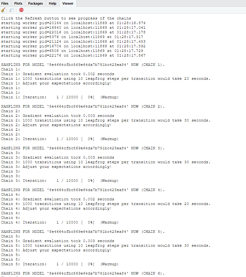
It runs extremely slow, 12hrs passed and still this is what i see:
Capture

Now I am aware I didn’t put any prior, could that be the issue?

model.1.1.prior<-get_prior(Y~X1+X2+X3+X4+X5+X6+(X1+X2+X3+X3+X4+X5+X5| Level_Variable),data=Mydataset,family = categorical(link = "logit", refcat = NULL)) #i am a bit confused at the output here; I haven't quite grasped how to use the information per se to get a proper prior.
#model.2.1.prior<-get_prior(Y~X1+X2+X3+X4+X5+X6+(X1+X2+X3+X3+X4+X5+X5| Level_Variable),data=Mydataset,family = sratio("logit")) .....the Y variable is ordinal but this doesn't work; I haven't investigated it more as of yet, due to the immense running hours.
SAMPLING FOR MODEL '662d5ea6d2b4caabd477e8a1873a1a11' NOW (CHAIN 1).
Chain 1: Rejecting initial value:
Chain 1:   Log probability evaluates to log(0), i.e. negative infinity.
Chain 1:   Stan can't start sampling from this initial value.
model1.1<-brm(Y~X1+X2+X3+X4+X5+X6+(X1+X2+X3+X3+X4+X5+X5| Level_Variable),data=Mydataset,family = categorical(link = "logit", refcat = NULL),prior = model.1.1.prior,control = list(max_treedepth = 15),warmup = 2500, iter = 10000, cores = getOption("mc.cores", 8),thin = 2, chains=8)

When I stopped the code after so many hours I got this message:

Warning message:
In system(paste(CXX, ARGS), ignore.stdout = TRUE, ignore.stderr = TRUE) :
  '-E' not found

>head(Mydataset)
         X1       X2      X3     Level_Variable       X4        Y             X5          X6
3      51         2        2            17               6000      1              45       24      
6      23         1        2             3               3000      4              24        15
7      50         1        4            14              10500      2            38        25  
14     55         2        2            15               2800      4             43      42
18     59         1        4             3               3600      3              30       18    
20     20         2        3            18               5000      4             30      23    

Y variable is a category taking values from 1 to 7. It could also be considered ordinal (which is a second step). However, I am guessing that the X4, X5, and X6 variables ( X5 max= 107) could be the case that it creates too many categories for each variable? The the issue is with the LVL_variable that has 21 levels?

apply(Mydataset,2,class)
            X1               X2                     X3                  Level_Variable          Y                      X5
         "numeric"          "numeric"          "numeric"          "numeric"          "numeric"          "numeric" 
            X6        
         "numeric"   

X1, X5, X4, X6 can be continuous (i.e Age, Payments), then X2, X3, Y are categoricals (1 to 4 i.e). The reason it takes too long is that probably I am definying something wrong. Maybe that model cannot be run with this technique? Any tips would be greatly appreciated.

`sessionInfo()
R version 4.1.1 (2021-08-10)
Platform: x86_64-w64-mingw32/x64 (64-bit)
Running under: Windows 10 x64 (build 19042)

Matrix products: default

Random number generation:
 RNG:     Mersenne-Twister 
 Normal:  Inversion 
 Sample:  Rounding 
 
locale:
[1] LC_COLLATE=English_United Kingdom.1252  LC_CTYPE=English_United Kingdom.1252   
[3] LC_MONETARY=English_United Kingdom.1252 LC_NUMERIC=C                           
[5] LC_TIME=English_United Kingdom.1252    

attached base packages:
[1] stats     graphics  grDevices utils     datasets  methods   base     

other attached packages:
[1] brms_2.16.1 Rcpp_1.0.7 

loaded via a namespace (and not attached):
  [1] nlme_3.1-152         matrixStats_0.61.0   xts_0.12.1           threejs_0.3.3        rstan_2.21.2        
  [6] tensorA_0.36.2       tools_4.1.1          backports_1.3.0      DT_0.19              utf8_1.2.2          
 [11] R6_2.5.1             DBI_1.1.1            mgcv_1.8-36          projpred_2.0.2       colorspace_2.0-2    
 [16] withr_2.4.2          tidyselect_1.1.1     gridExtra_2.3        prettyunits_1.1.1    processx_3.5.2      
 [21] Brobdingnag_1.2-6    curl_4.3.2           compiler_4.1.1       cli_3.1.0            shinyjs_2.0.0       
 [26] colourpicker_1.1.1   posterior_1.1.0      scales_1.1.1         dygraphs_1.1.1.6     checkmate_2.0.0     
 [31] mvtnorm_1.1-3        ggridges_0.5.3       callr_3.7.0          stringr_1.4.0        digest_0.6.28       
 [36] StanHeaders_2.21.0-7 minqa_1.2.4          base64enc_0.1-3      pkgconfig_2.0.3      htmltools_0.5.2     
 [41] lme4_1.1-27.1        fastmap_1.1.0        htmlwidgets_1.5.4    rlang_0.4.12         rstudioapi_0.13     
 [46] shiny_1.7.1          farver_2.1.0         generics_0.1.1       zoo_1.8-9            jsonlite_1.7.2      
 [51] gtools_3.9.2         crosstalk_1.1.1      dplyr_1.0.7          distributional_0.2.2 inline_0.3.19       
 [56] magrittr_2.0.1       loo_2.4.1            bayesplot_1.8.1      Matrix_1.3-4         munsell_0.5.0       
 [61] fansi_0.5.0          abind_1.4-5          lifecycle_1.0.1      stringi_1.7.5        MASS_7.3-54         
 [66] pkgbuild_1.2.0       plyr_1.8.6           grid_4.1.1           parallel_4.1.1       promises_1.2.0.1    
 [71] crayon_1.4.1         miniUI_0.1.1.1       lattice_0.20-44      splines_4.1.1        ps_1.6.0            
 [76] pillar_1.6.4         igraph_1.2.7         boot_1.3-28          markdown_1.1         shinystan_2.5.0     
 [81] reshape2_1.4.4       codetools_0.2-18     stats4_4.1.1         rstantools_2.1.1     glue_1.4.2          
 [86] V8_3.4.2             RcppParallel_5.1.4   vctrs_0.3.8          nloptr_1.2.2.2       httpuv_1.6.3        
 [91] gtable_0.3.0         purrr_0.3.4          assertthat_0.2.1     ggplot2_3.3.5        xfun_0.27           
 [96] mime_0.12            xtable_1.8-4         coda_0.19-4          later_1.3.0          rsconnect_0.8.24    
[101] tibble_3.1.5         shinythemes_1.2.0    tinytex_0.34         gamm4_0.2-6          ellipsis_0.3.2      
[106] bridgesampling_1.1-2`

There are certainly a few things that might help to get the model running faster. To your point, part of the problem could just be that the model is misspecified; however, there are some options that you’ve set that are going to also increase the time to get your results.

It’d be great to know what you’ve already tried with this model that prompted you to change the default options for brms. I see that you’ve increased the max treedepth and adapt delta (both of these are going to increase fitting time), but the defaults for those options are usually pretty good for a lot of regression models. I see that you’re also doing 10000 iterations and then also thinning by 2. Unlike many other Bayesian estimators (e.g., JAGS, BUGS), Stan generally doesn’t need that many iterations or any thinning to get converging chains.

I’m not sure why you’re fitting on 8 chains (generally 4 is sufficient). I’d suggest, particularly if speed is an issue, fitting on 4 chains but using the threading option in brms to use those extra 4 cores more efficiently. There are more details about that here: Running brms models with within-chain parallelization. The big piece though is that you’d add something like the following to your brm call: ...backend = "cmdstanr", threads = threading(4)). Another thing that might speed up your estimation is to use a QR decomposition: brm(bf(y ~ x1 + x2 + x3 + x4 + x5 + (x1 + x2 + x3 + x4 + x5 | Level_Variable), decomp = "QR"), ...). I can’t recall off the top of my head whether QR decompositions are supported for categorical/ordinal models, but worth a shot regardless.

I’m not sure what you mean by those variables having too many categories for each variable. One thing I notice about your predictor variables are that they are all on pretty different scales (particularly X4-6). That can make the posterior distribution harder to sample, especially if there aren’t any priors. You can either specify some variable specific priors (i.e., priors on each predictor with appropriate scale to that predictor), or you can try rescaling your predictors (e.g., standardizing them).

Given that your outcome variable is given by a variable ranging from 1-7 and could be considered ordinal (sounds Likert-y to me), I suspect that it actually is ordinal; however, the details of what you’re trying to do are not in this first question, so it’s tough to say exactly whether your outcome is perhaps something other than categorical.

This really depends more on how many observations you have. I don’t see anywhere where you clarify what the size of your sample is. You can have really large numbers of levels in random effects as long as you have sufficient observations of cases in those levels. If it’s a question, though, you can always run the model without the random effects. Indeed, there’s a lot of merit to trying to run simpler versions of the model because then you can (a) actually get some results but more importantly (b) see what variables contribute to specific problems or concerns. In terms of your question about whether a categorical model is most appropriate, getting some results allows you to perform posterior predictive checks, via ppc(fit, type = "bars"), to see whether that likelihood is an appropriate specification for your data.

If I’m reading your output of apply(Mydataset, 2, class), then those variables are numeric (as is your Y and Level_Variable), not categorical. If you want brms to treat them as categorical, then you need to specify those as factors or ordered factors.

This can be safely ignored. There are several posts on this forum about it, and it’s totally innocuous.

Generally speaking, it’d be helpful for us to know more about your data, what you’ve tried, and what you’re trying to answer with the model. There are a lot of very interesting and powerful models that can be fit in brms, but it’s hard to make recommendations about what kinds of things to try without knowing what the end goal is or what the data look like.

1 Like

Hello! THank you for the response. The data are shown as numeric because I changed the class to them to numeric (apply(data,2,as.numeric) because at the time, I couldn’t run anything cause everything was considered as a character variable.

The data are pretty small; 522 observations and 7 variables (X1:6 and Y). X2 and X3 and Y are variables that are a response from a questionaire 1 to 7 is the range. The LVL is another categorical with 21 levels. X4, x6, and X1 are continuous positives (hours,age/income for example), and X5 is an index variable from a combination of categorical variables, but I would consider it more like a continuous as well. The end goal is to estimate the level of Y (1 to 7) based on the effects from X1:X6. Can X1:X6 put an individual to a specific category with a good accuracy?

First, when fitting complex models it is generally good practice to build your model up in some principled way because it is easier to debug a simpler model. A multinomial logistic regression model with six varying slopes is going to be extremely costly in terms of computation and makes some pretty extreme demands of your data unless you have a fairly large number of observations.

Second, as @wgoette pointed out, you want your inputs to all be on roughly the same scale because it makes it easier for the sampler to explore the parameter space. There are various ways to go about this and you can either center your interval predictors at their group means and either divide by two standard deviations, some numeric constant (there are varying opinions on which is more appropriate), or employ a QR decomposition.

Third, you’re going to want to specify at a minimum some weakly informative priors on your parameters to aid in model convergence. In the context of brms, consider the following example

# Specify the formula for the model
multilogit_vote <- bf(
  vote_choice ~ female + age_gmc + unemployed + income_gmc + university + time_gmc + female:time_gmc + (1 + income_gmc | state_jj),
  family = categorical(link = "logit", refcat = "Democrat"),
  decomp = "QR"
)

# Specify Priors for the model
priors_multilogit_vote <-
  prior(normal(0, 10), class = "Intercept", dpar = "muOther") +
  prior(normal(0, 1), class = "b", dpar = "muOther") +
  prior(lkj(4), class = "cor", dpar = "muOther") +
  prior(exponential(0.8), class = "sd", dpar = "muOther") +
  prior(normal(0, 10), class = "Intercept", dpar = "muRepublican") +
  prior(normal(0, 1), class = "b", dpar = "muRepublican") +
  prior(exponential(0.8), class = "sd", dpar = "muRepublican") +
  prior(lkj(4), class = "cor", dpar = "muRepublican")

# Fit the multinomial logistic regression mode----
multilogit_vote_fit <- brm(
  formula = multilogit_vote,
  data = cces_ts,
  prior = priors_multilogit_vote,
  iter = 3000,
  warmup = 1500,
  inits = 0.1,
  chains = 6,
  cores = 12,
  seed = 123,
  control = list(
    adapt_delta = 0.90,
    stepsize = 0.1,
    max_treedepth = 12
  ),
  backend = "cmdstanr",
  refresh = 10,
  save_model = "Models/CCES_Vote_MultiLogit.stan",
  file = "Models/CCES_Vote_MultiLogit"
)

Using cmdstanr as a backend instead of rstan will allow you to take advantage of the latest version of stan which has undergone a lot of improvements in performance compared to the older version rstan (assuming you’re using the cran version) relies on at this time.

If you are new to Bayesian inference and brms, I strongly recommend checking out @Solomon’s amazing resources Statistical rethinking with brms, ggplot2, and the tidyverse: Second edition and Doing Bayesian Data Analysis in brms and the tidyverse on data analysis with brms. Also, the recently released online version of Bayes Rules! An Introduction to Bayesian Modeling with R provides an amazing and very user-friendly introduction to Bayesian inference

3 Likes

Broadly, I echo what @ajnafa had to say, and I think the example he provided will be a good resource for you. There are a few things I wanted to add in based on what you responded.

This can be handled in R with the as.factor() function. Sounds like when you imported the data into R, the data were initially strings/text. This comes up a lot, so here’s an example of how to deal with that in R. Say that you have a variable for Sex that is recorded as either “Male” or “Female.” Just importing that data in R, it will think that this is a character variable since it contains text. You can tell R that this is actually a factor variable as follows: data$Sex <- factor(data$Sex, levels = c("Male", "Female"), labels = c("Male", "Female") or even more simply as data$Sex <- as.factor(data$Sex).

This is still not really clear in terms of what the responses mean. For example, is someone rating their familiarity with something or how much they agree with a statement? Is the person asking to select their favorite option or a statement they agree with most?

How many observations are in each level? If the full sample is equally distributed within these levels, then that’s ~25 observations/level. As @ajnafa observed, this is already a fairly costly computation, and the accuracy of the random effects estimates may be fairly low if some of those levels don’t have many observations. As I noted, it’d be helpful for us to know the context of your analysis. Is this an experimental study where people were assigned to these levels? Are these levels representing natural clustering of observations (e.g., by region, neighbhorhood, etc)? Are they reflecting repeated observations of the same 21 people over a period of time?

Just to be clear, this sounds like the goal of the model is predictive accuracy: that is, the desired end state is to produce a model that accurately predicts what response (from 1 to 7) a person will provide to some questionnaire. In these cases, it’s really important to think about how your data are generated, meaning what processes occur that cause the original data you observed to be the way they are. Really thinking critically about how someone selects the response they have and why you think the predictors you have are predictors of this process can help to shed light on the kind of model you should be building. For example, there are several ordinal models and each makes different assumptions about how to think about the underlying process of choosing a 3 over a 2 or 4. Multinomial logistic regression (i.e., regression with the categorical likelihood) does not make those same kinds of assumptions about the underlying process. You probably want to begin with a model that matches your understanding of the data generation process and then perform your model checks to see whether that was accurate or what needs to be improved

2 Likes

Thank you for the amazing responses!

@ajnafa Just a clarification; the priors you have set up in the priors_multilogit_vote are respective to the formula you have set up right? i.e the unemployed have a prior lkj(4) (the 4 refers to the number of levels?).

In response to @wgoette questions about the number of obs on some levels, sadly on average there are 10 obs per level. There are 21 levels, and some have 1,2 obs, and some have 20, but on average its 10. I am going to integrate some in onelevel.

Sadly I have no impact on the way the data have been collected from the questionaire.

I’ll let @ajnafa clarify the priors generally; however, I can at least let you know that the lkj(4) prior does not have to do with the number of levels. The LKJ prior has a shape parameter (usually \eta) that affects it’s behavior. You can read more about the prior here: 25.1 LKJ correlation distribution | Stan Functions Reference. Typically, the default \eta shape parameter is 1 (i.e., lkj(1)) since this is roughly uniform over correlation matrices.

I’m not sure that any of the things that we’ve recommended/suggested on this thread have required alternative data collection. I think the biggest thing that’s come up is just that you haven’t shared what the variables actually are, just how they’re measured. Without knowing what is being modeled, it’s very hard to try to think about how a model should be built. To me, the biggest question is whether you need a categorical model at all. My experience is that questionnaire data are usually ordinal, and ordinal models may be more straightforward to implement than the categorical model; however, without actually knowing what the questionnaire is or the kinds of items, all we can do is point out some things that might make the categorical model run faster

@wgoette Gotcha!

The response variable is an ordinal (1 to 7 levels) number of times exercising.
The X1 (Age), X2 (gender), X3 (location exercising takes place), X4 (income but I converted to a categorical), X5 (stress in their lives <-that probably I should convert to ordinal), X6 work hours and Level-Variable (industry they belong). I want to figure out if X1-6 can predict the amount of time one would be exercising (in the future i want to use this to relate to mental health, but haven’t worked that part yet). Is that what you meant @wgoette ?

1 Like

That’s very helpful to know!

The categorical model does not seem like it would necessarily be appropriate for your outcome since it is ordinal in nature. There is an excellent instructional paper on ordinal regression using brms (link here). Based on your outcome, a reasonable place to start might be sequential model because in order to exercise, for example, 5-6 times per week one must also necessarily have exercises 1-3 times per week (hence the ordinal nature of the responses are sequential).

My guess is that the model will run faster and have less convergence issues if you do an ordinal regression. Still, be sure to check the posterior predictive plots, and it’s going to be good for you to still specify priors.

A note on a few of your predictors. You may still consider scaling some of the continuous variables. That’s not necessary, but it does make specifying the priors easier and can help make the posterior easier to sample from. I’d also double check that you have specified the data types correctly for your predictors in R so that brms knows what kind of variables they are. Seems like X1 is numeric, X2 is a factor, X3 is a factor, X4 is an ordered factor, X5 is numeric (or an ordered factor if you make it ordinal), X6 is numeric, and Level is a factor.

Not sure how you could make this categorical. The simplest categorization I can think of would be like a median split, and even then, that is ordinal since one group is necessarily ranked higher on the variable than the other. Income data can be heavily skewed and have very long tails, but generally log transformations of the variable make income a fairly well-behaved predictor. I’d err on including it as a continuous, numeric variable (probably log-transformed) and then trying to make it ordinal if it starts to cause problems in the model estimation.

I’d also just throw out there that you can wrap any ordinal predictors in the mo() function from brms. This is just a brms-specific helper to estimate monotonic effects of predictors (read more here). The alternative is to specify ordinal predictors as ordered factors in R and then make sure you’re using your desired contrast coding for ordered variables (the same is true for factor variables)

I was thinking to make the income one like 1 category (low income), 2nd Category middle class, upper class something like that.

I am a bit unsure how to specify the model. I think I have defined it well; not sure, and for the priors I tried using the get_prior command but it was quite confusing to interpret the output.

This would be ordinal since Category 1 < Category 2 < Category 3. Ordinal variables are just those that are non-continuous or unequally distanced but have some degree of ordering.

Could you share the model syntax that you tried? Based on the old code, I’d think something like this would work:

model <- brm(bf(Y ~ X1 + X2 + X3 + X4 + X5 + X6 + (X1 + X2 + X3 + X4 + X5 + X6 | Level_Variable),
                decomp = "QR"),
             family = sratio(), data = Mydataset)

This assumes no priors (not recommended) and that you don’t need to tweak any of the default settings. If it returns any convergence errors, then I’d suggest trying it without the random slopes part since that’s a lot of random effects that you’re estimating. If there are still issues, then I’d think that it has something to do with the predictors and the potentially disparate scaling of those predictors (that’s assuming that you’ve used priors – if you didn’t use priors, then adding reasonable priors would be the place to begin)

That’s exactly what i tried with out priors. I tried the get_prior to find what priors I should use, but I couldn’t understand the outcome properly.

I recommend reading through the ordinal regression in brms tutorial that I linked to in an earlier post. There is a relatively simple and straightforward example of setting priors there.

I do not think that you need to adjust most of the priors that you get from the get_prior() function. The biggest thing to change would be the priors for the regression coefficients (class = 'b') and then maybe the intercept (class = 'Intercept')

----EDIT (Extra Question)----
You said that you tried the model I gave as an example. What was the result? Were there errors or anything?

i have never finished it running to be honest. I stopped it cause 5 days had passed and it was still at 30%. Now when i tried again i was getting this:

Compiling Stan program...
When you compile models, you are also contributing to development of the NEXT
Stan compiler. In this version of rstan, we compile your model as usual, but
also test our new compiler on your syntactically correct model. In this case,
the new compiler did not work like we hoped. By filing an issue at
https://github.com/stan-dev/stanc3/issues with your model
or a minimal example that shows this warning you will be contributing
valuable information to Stan and ensuring your models continue working. Thank you!
This message can be avoided by wrapping your function call inside suppressMessages()
 or by first calling rstan_options(javascript = FALSE).
Error in context_eval(join(src), private$context, serialize) : 
  248,Stack_overflow,-9


Warning messages:
1: Rows containing NAs were excluded from the model. 
2: In system(paste(CXX, ARGS), ignore.stdout = TRUE, ignore.stderr = TRUE) :
  '-E' not found
Error in sink(type = "output") : invalid connection

Couple things here to clarify.

First, are you getting this error with other brms models? I’ve seen several posts on this forum recently on the sink() and Stack_overflow errors, so you may try searching for that to see if there’s something you need to adjust in order to get Stan to run in parallel. That’s outside of my skill set, though, and I can’t tell you much more than the fact that I’ve seen some of these issues on the forum recently.

This seems highly unusual to me, and probably is sign that the model is misspecified. It’d be helpful to see exactly what you ran that was taking so long. My guess here is that the random effects are part of the problem. I don’t really know enough about your data and its collection to say, but I don’t really know that Level_Variable is a grouping factor – it sounds more like a categorical predictor. The random effects are going to add complexity to the model, and I think at this point you just need a model that gives you some kind of result so that you can figure out how to go from there.

Generally speaking, it’s better to begin with the simplest models first and then work up to the most complicated so that you can tell what causes the model to break (if it breaks at all). Even better practice is beginning with simulation-based calibrations of the model to ensure that your specification and priors are behaving as you desire. There are several resources on simulation-based calibration, if you’re interested: 27 Simulation-Based Calibration | Stan User’s Guide, https://statmodeling.stat.columbia.edu/2021/09/03/simulation-based-calibration-some-challenges-and-directions-for-future-research/, Simulation Based Calibration, and R package for implementing simulation based calibration using rank statistics • sbcrs).