Chains initialisation explode for large T in dynamic factor model

99_bdfm_tester.R (1.3 KB)
bdfm_tester.stan (1.1 KB)

Hello,
I have recently started using Stan for estimating Dynamic Factor Models. Following some of the (very few) examples found here and elsewhere, I coded up a simple DFM that I wanted to test on simulated data. I specified the factors in the transformed parameters bloc and sampled from their errors, as I understand is better than having them directly in the model bloc. I attach both stan code and R script to simulate some data and feed them to Stan.

The estimation of the model - if well identified - works generally well, although I noticed a strange behaviour when using multiple chains, as illustrated in the picture below (apologies for the low res).

In short for a total of T periods of time in the model, the initial point for some chains progressively explodes to unreasonable values as t grows towards T. I don’t understand if it is a result of how I modelled the factors or an unintended side effect.

Typically, increasing the number of iterations (or setting init=0) solves the issue, especially with smaller models, although this becomes impractical and cumbersome with larger, more complicated models.

Any suggestions or explanations about this behaviour?

Given that there are reasonably constrained priors on ar_facts and eps_s, my guess sis that the multiplicative form of the factors is just stacking up given that it’s a multiplicative time series. The reason I say that is that you can see the scale grow on your diagram. One thing you can do if you want to keep the time series of factors stationary is constrain ar_facts more strongly than with a normal(0, 10) prior. As is, if ar_facts = 5, then each step in the time series is going to scale everything by 5, which grows very quickly.

The model is degenerate here in that Y[:, 1] is not being modeled. You can just add a distribution for it up front if you want a fully generative model.

P.S. There are a few ways to dramatically speed up this code. You don’t ever need to create a diagonal covariance matrix explicitly—you can just use the univariate normal to get the same effect, because if sigma and y are vectors, then these two forms are equivalent (up to a constant):

y ~ normal(mu, sigma)
==
y ~ multi_normal(mu, diag_matrix(sigma));

Thus, you an replace:

  1. You can replace
cov_matrix[K] cov_f = identity_matrix(K);
...
for (t in 1:T) {
  eps_s[:, t] ~ multi_normal(mu_f, cov_f);
}

with something that just gives each entry in the matrix a normal prior with location mu_f and scale 1.

to_vector(eps_s) ~ normal(mu_f, 1);
  1. You can replace
cov_matrix[N] cov_y = diag_matrix(sigma_y);
...
for (t in 2:T) {
  Y[:, t] ~ multi_normal(loadings*factors[:,t], cov_y);
}

with

matrix[N, T] loadings_factors = loadings * factors;
for (n in 1:N) {
  Y[n] ~ normal(loadings_factors[n], sigma_y[n]);
}

Thanks @Bob_Carpenter, it was more or less the same intuition I had, though the issue seem to persist even with tighter priors on the (V)AR part: the divergence of factors is way less pronounced but still there. Letting the iterations grow brings the distribution back to more reasonable values though.

Also, I added the coding tweaks you proposed and indeed the code runs in a fraction of the time, thanks a million for saving me a ton of time!

I played around with the code and tried a few things. One thing that seems to help to me is to constrain the factors to be stationary or at most random walk, by imposing them to be between -1 and 1. That should help rule out the more explosive behaviour, and I feel it’s not an unreasonable restriction in this type of setting.

matrix<lower=-1,upper=1>[K, K]           ar_facts;

This already imposes a stronger regularization than the normal(0, 10) prior you already have, but you may want to tweak that prior further.

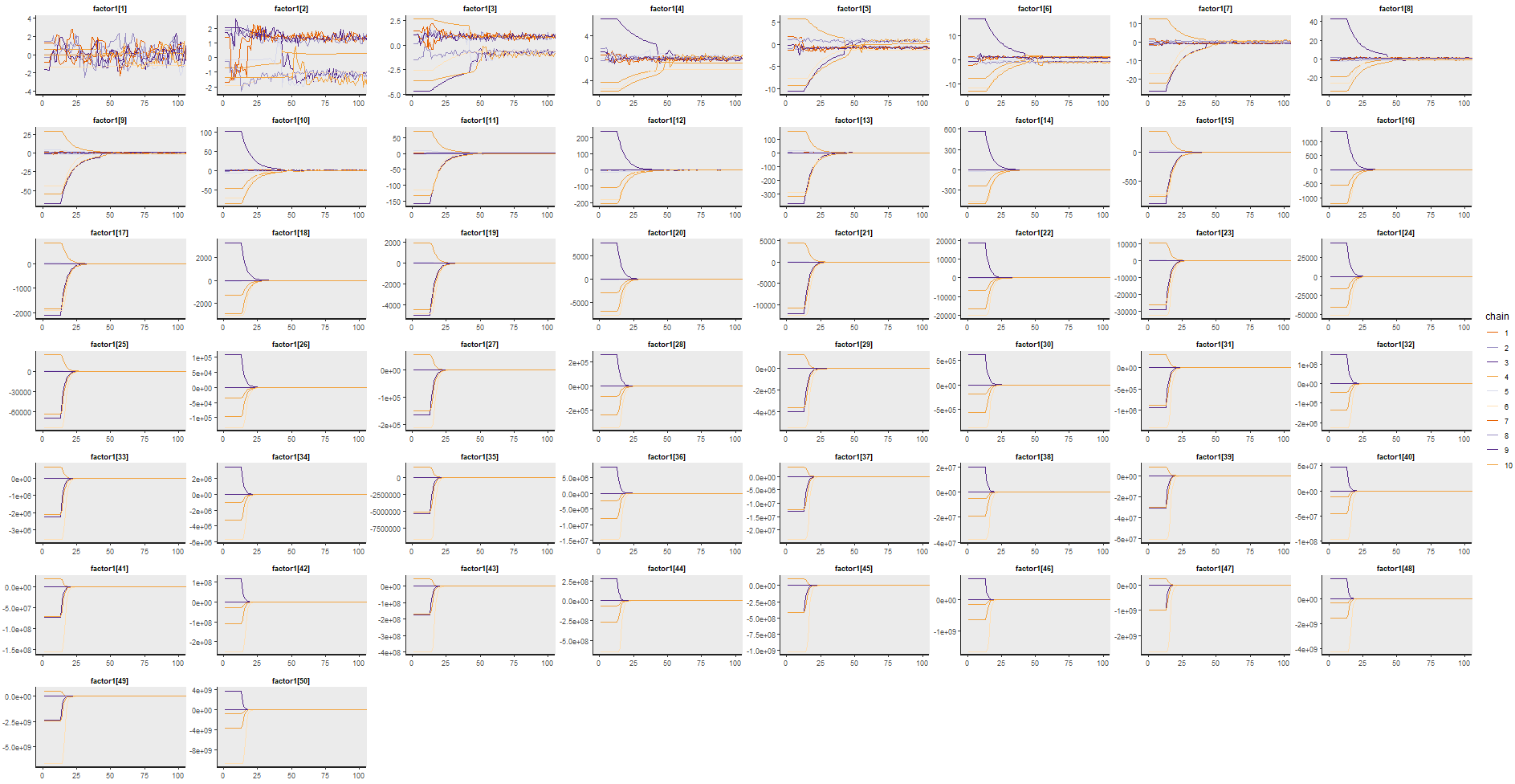
With this approach, I generally get good behaviour, although indeed a couple of misbehaved chains seem to have the top loads close to 0 and get stuck there. Then the remaining variables get the wrong side in their loadings, and thus the estimated factors also have the wrong sign, but “correct” with a sign switch. I tried to ensure I was running the model with strong loadings on the first variable to ensure identifiability, as otherwise it’s easier for that loading to be estimated as small positive 0 and then the remaining variables to end up in different chains on different sides of positive and negative. And I also played with simulating data with ar_facts with a larger number (0.7), as I wondered if -0.1 is too weak for any discernible factor structure to be estimated. Still, this did not seem to be enough to get good results every time I ran with your example (N = 5, T = 300).

This is a strange conjecture, and maybe I can’t explain it clearly. I think the main issue is the top load getting stuck at 0, and the HMC being unable to move away from that. I wonder if what’s happenning is the following. The top load must be positive due to the cholesky_factor_cov constraint you impose, I think. And in simulations, I ensured that it was strongly positive (among the largest absolute values). Suppose that the estimation of the top load starts close to 0. What may happen as the DFM grows is that the model is still able to have a factor that is driving all the other N-1 variables reasonably well, but with the opposite sign, and will just ignore that first variable, imagining it to have a very small loading close to 0. As this has still a high likelihood (as the single factor can explain N-1 variables), it’s hard for it to move away from 0, as that would require a large move if the first_load is high and would require a sign switch for all the other loadings and the factors. An additional signal in this direction is that if I simulate data with all positive factors AND I restrict bottom_loads to be positive, the estimation avoids the R-Hat and E-BFMI issues (although in my only attempt it still had a small number of divergent transitions). However, in practice this may be hard to ensure, or would require you to do some pre-processing that may not even be obvious how to do.

I hope these are useful clues. If you learn anything about the topic, please keep posting, as I’m also interested in estimating these models in Stan.

1 Like

Not sure how helpful it is but I’ve played around a lot with latent dynamic factor models lately so I think I can offer some advice.

First, it is often necessary to impose a specific set of constraints on the factor loadings to avoid identifiability issues. Of course these constraints can mean that different chains have different solutions, but there is a convenient trick one can use in generated quantities to sign correct the loadings / factors (see a detailed discussion of both issues in this Discourse post).

Second, if you hope to eventually change from AR to VAR dynamics, you will certainly find some explosive solutions due to the fact that, proportionally, the vast majority of possible parameter space typically leads to nonstationarity in VARs (see this paper by Sarah Heaps for more details). Sarah provides some useful functions that can be implemented in Stan to enforce stationarity of the VAR while allowing for more informed priors to be used, so I’d recommend you have a look there if VARs are your goal.