I would like to know if anyone has translated an example from Bayesian Data Analysis (3rd edition) to Stan. That example is Stratified sampling in pre-election polling, chapter 8, page 207. I know that there is a repository where you can find examples from BDA3 in Stan (here, but there are no examples from chapter 8) and I could do that, but I prefer to ask before I begin.
Let’s begin with the nonhierarchical model. I will be using python. If you want to follow along with the code, first go here and download the file as .txt. I called it cbs_survey.txt.
Import some libraries:
import numpy as np
import matplotlib.pyplot as plt
import pystan
import pandas as pd

plt.style.use('seaborn-darkgrid')
plt.rc('font', size=12)
It is a survey of 1447 people, so:
participants = 1447
data = pd.read_csv('cbs_survey.txt', sep=' ', skiprows=2, skipinitialspace=True, index_col=False)
print(data)
We need the number of people of each region and each candidate.
data_obs = data[['bush', 'dukakis', 'other']].to_numpy()
print(data_obs)
And a variable called proportion:
proportion = data['proportion'].to_numpy() * participants
print(proportion)
And another variable:
valores = data_obs[:, :] * proportion.reshape(16, -1)
valores = np.round(valores)
np.sum(valores) # Check if the sum is equal to 1447
Now, Stan
model_non_hier="""
data {
  int<lower=0> N;
  int<lower=0> n;
  int y_obs[N, n];
  vector[n] alpha;
}

parameters {

  simplex[n] theta[N];
}

model {

  for (i in 1:N)
    theta[i] ~ dirichlet(alpha);

  for (i in 1:N)
    y_obs[i] ~ multinomial(theta[i]);
}

"""
Now:
stan_model = pystan.StanModel(model_code=model_non_hier)
data2 = {'N': 16,
       'n': 3,
       'alpha': [1,1,1],
       'y_obs': valores.astype(int)}
fit = stan_model.sampling(data=data2)
The output is very long.
print(fit.stansummary(digits_summary=5))
Inference for Stan model: anon_model_2a28c5090c429737936718a5aee45413.
4 chains, each with iter=2000; warmup=1000; thin=1;
post-warmup draws per chain=1000, total post-warmup draws=4000.

              mean se_mean     sd   2.5%    25%    50%    75%  97.5%  n_eff   Rhat
theta[1,1]  0.3007  0.0006 0.0643 0.1805 0.2566 0.2987 0.3413 0.4357   8933 0.9995
theta[2,1]  0.4902  0.0008 0.0726 0.3454 0.4426 0.4907 0.5382 0.6296   7457 0.9997
theta[3,1]  0.4648  0.0003 0.0379 0.3918 0.4387 0.4640 0.4902 0.5415   9417 0.9995
theta[4,1]  0.4587  0.0006 0.0566 0.3484 0.4198 0.4589 0.4974 0.5708   7798 0.9993
theta[5,1]  0.4011  0.0007 0.0690 0.2691 0.3541 0.3999 0.4479 0.5394   9671 0.9993
theta[6,1]  0.4424  0.0005 0.0510 0.3418 0.4083 0.4422 0.4758 0.5441   8823 0.9992
theta[7,1]  0.5041  0.0005 0.0467 0.4125 0.4723 0.5041 0.5361 0.5958   8730 0.9993
theta[8,1]  0.5474  0.0004 0.0412 0.4684 0.5191 0.5470 0.5772 0.6272   7904 0.9992
theta[9,1]  0.5420  0.0011 0.0984 0.3488  0.474 0.5443 0.6117 0.7277   7048 0.9994
theta[10,1] 0.4640  0.0005 0.0495 0.3675 0.4304 0.4641 0.4974 0.5617   8140 0.9994
theta[11,1] 0.5103  0.0006 0.0491 0.4110 0.4786 0.5098 0.5430 0.6038   6471 1.0000
theta[12,1] 0.5513  0.0004 0.0357 0.4815 0.5270 0.5506 0.5749 0.6215   7018 0.9993
theta[13,1] 0.4868  0.0008 0.0796 0.3304 0.4328 0.4865 0.5421 0.6381   8040 0.9992
theta[14,1] 0.5245  0.0006 0.0550 0.4146 0.4872 0.5255 0.5615 0.6307   7609 0.9998
theta[15,1] 0.5362  0.0004 0.0438 0.4496 0.5067 0.5373 0.5662 0.6197   9523 0.9996
theta[16,1] 0.5467  0.0005 0.0553 0.4364 0.5082 0.5471 0.5851 0.6519   8899 0.9997
theta[1,2]  0.5990  0.0008 0.0698 0.4569 0.5527 0.6008 0.6479 0.7298   7472 0.9993
theta[2,2]  0.4687  0.0008 0.0729 0.3284 0.4189 0.4679 0.5171 0.6174   7076 0.9997
theta[3,2]  0.4118  0.0004 0.0377 0.3386 0.3867 0.4115 0.4376 0.4858   8076 0.9997
theta[4,2]  0.5137  0.0006 0.0574 0.4014 0.4739 0.5140 0.5538 0.6282   7946 0.9994
theta[5,2]  0.4793  0.0007 0.0693 0.3462 0.4325 0.4794 0.5265 0.6144   8717 0.9993
theta[6,2]  0.4439  0.0005 0.0504 0.3453 0.4107 0.4431 0.4768 0.5447   8078 0.9993
theta[7,2]  0.3863  0.0004 0.0447 0.2973 0.3561 0.3854 0.4156 0.4760   8224 0.9993
theta[8,2]  0.3377  0.0004 0.0393 0.2636 0.3094 0.3373 0.3652 0.4153   7598 0.9993
theta[9,2]  0.2921  0.0010 0.0896 0.1357 0.2273 0.2865 0.3510 0.4831   7374 0.9993
theta[10,2] 0.4042  0.0005 0.0490 0.3086 0.3713 0.4038 0.4377 0.4997   7401 0.9997
theta[11,2] 0.4014  0.0006 0.0489 0.3059 0.3680 0.4007 0.4339 0.5005   6078 0.9996
theta[12,2] 0.3511  0.0004 0.0350 0.2808 0.3278 0.3510 0.3736 0.4225   7039 0.9996
theta[13,2] 0.4595  0.0009 0.0794 0.3089 0.4043 0.4587 0.5137 0.6184   7402 0.9993
theta[14,2] 0.3507  0.0006 0.0542 0.2478 0.3126 0.3489 0.3875 0.4623   8022 0.9994
theta[15,2] 0.3691  0.0004 0.0427 0.2854 0.3405 0.3685 0.3975 0.4549   7822 0.9995
theta[16,2] 0.3600  0.0005 0.0532 0.2594 0.3234 0.3589 0.3969 0.4663   8431 0.9996
theta[1,3]  0.1002  0.0004 0.0423 0.0333 0.0692 0.0952 0.1255 0.1975   7723 0.9993
theta[2,3]  0.0410  0.0003 0.0285 0.0051 0.0201 0.0347 0.0552 0.1128   6573 0.9999
theta[3,3]  0.1233  0.0002 0.0246 0.0793 0.1056 0.1223 0.1395 0.1750   8132 0.9999
theta[4,3]  0.0275  0.0002 0.0188 0.0032 0.0135 0.0236 0.0370 0.0749   6783 0.9997
theta[5,3]  0.1195  0.0005 0.0449 0.0459 0.0864 0.1152 0.1466 0.2226   8130 0.9995
theta[6,3]  0.1135  0.0003 0.0321 0.0577 0.0904 0.1112 0.1334 0.1824   7675 0.9992
theta[7,3]  0.1095  0.0003 0.0292 0.0603 0.0880 0.1073 0.1281 0.1701   7200 0.9994
theta[8,3]  0.1147  0.0003 0.0256 0.0689 0.0966 0.1132 0.1315 0.1691   7493 0.9994
theta[9,3]  0.1658  0.0009 0.0735 0.0503 0.1113 0.1582 0.2113 0.3322   6146 0.9995
theta[10,3] 0.1317  0.0004 0.0340 0.0724 0.1076 0.1297 0.1528 0.2042   7260 0.9997
theta[11,3] 0.0881  0.0003 0.0282 0.0409 0.0676 0.0855 0.1058 0.1517   7555 0.9993
theta[12,3] 0.0975  0.0002 0.0226 0.0583 0.0815 0.0959 0.1120 0.1456   6503 0.9997
theta[13,3] 0.0535  0.0004 0.0371 0.0060 0.0262 0.0458 0.0723 0.1464   6138 0.9994
theta[14,3] 0.1247  0.0004 0.0364 0.0619 0.0987 0.1217  0.148 0.2014   6789 0.9994
theta[15,3] 0.0946  0.0003 0.0266 0.0490 0.0754 0.0919 0.1113 0.1525   7251 0.9991
theta[16,3] 0.0932  0.0003 0.0315 0.0409 0.0706 0.0900 0.1123 0.1651   7889 0.9993
lp__       -1.4149e3  0.1127 4.2446-1.4241e3-1.4175e3-1.4145e3-1.4118e3-1.4076e3   1418 1.0038

Samples were drawn using NUTS at Tue Jul 30 17:33:35 2019.
For each parameter, n_eff is a crude measure of effective sample size,
and Rhat is the potential scale reduction factor on split chains (at
convergence, Rhat=1).
Let’s reproduce Figure 8.1(a).
samples = fit.extract(permuted=True)['theta']
print(sample.shape)

diff3 = []

for i in range(16):
    result3 = samples[:, i, 0] - samples[:, i, 1]
    diff3.append(list(result3))

diff3 = np.asarray(diff3)
res3 = np.sum(diff3.T * proportion / np.sum(proportion), axis=1)

plt.figure(figsize=(10, 6))
_, _, _ = plt.hist(res3, bins=20, edgecolor='w', density=True)
plt.show()

Nice!
Now the book goes to the hierarchical model (page 209).
As an aid to constructing a reasonable model, we transform the parameters to separate
partisan preference and probability of having a preference:\alpha_{1j} = \dfrac{\theta_{1j}}{\theta_{1j} + \theta_{2j}},
\alpha_{2j} = 1 - \theta_{3j}.
To get \alpha_{1j} and \alpha_{2j}:
alpha_2j = np.round((1 - data['other'].to_numpy()) * data.proportion.to_numpy() * participants)
print(alpha_2j)

alpha_1j = valores[:, 0] / (valores[:, 0] + valores[:, 1]) * data.proportion.to_numpy() * participants
print(alpha_1j)

new_values = np.round(np.stack([alpha_1j, alpha_2j], axis=1))
print(new_values)
With Stan:
model_hier="""
data {
  int<lower=0> N;
  int<lower=0> n;
  int post[N, n];
}

parameters {
  vector[n] mu;
  cholesky_factor_corr[n] L;
  simplex[n] alphas[N];
  vector[n] beta[N];

}

transformed parameters{

  vector[n] theta[N];

  for (i in 1:N)
    theta[i] = inv_logit(beta[i]);

}

model {

  L ~ lkj_corr_cholesky(3.0);

  mu ~ cauchy(0, 5);

  beta ~ multi_normal_cholesky(mu, L);


  for (i in 1:N)
    alphas[i] ~ dirichlet(theta[i]);

  for (i in 1:N)
    post[i] ~ multinomial(alphas[i]);

}

generated quantities {

  corr_matrix[n] Sigma;
  Sigma = multiply_lower_tri_self_transpose(L);

}

"""
I have to say I am not happy about the code.
stan_model2 = pystan.StanModel(model_code=model_hier)
data3 = {'N': 16,
         'n': 2,
         'post': new_values.astype(int)}
fit2 = stan_model2.sampling(data=data3, algorithm='HMC', iter=4000, verbose=True)
Of course, there are warnings:
WARNING:pystan:n_eff / iter below 0.001 indicates that the effective sample size has likely been overestimated
WARNING:pystan:Rhat above 1.1 or below 0.9 indicates that the chains very likely have not mixed
WARNING:pystan:Skipping check of divergent transitions (divergence)
WARNING:pystan:Skipping check of transitions ending prematurely due to maximum tree depth limit (treedepth)
The output is very long
print(fit2.stansummary(digits_summary=5))
Inference for Stan model: anon_model_958bb8552d6652a8814e6044bd42f4a8.
4 chains, each with iter=4000; warmup=2000; thin=1;
post-warmup draws per chain=2000, total post-warmup draws=8000.

               mean se_mean     sd   2.5%    25%    50%    75%  97.5%  n_eff   Rhat
mu[1]       2.2705e1  8.01884.6381e1 1.1962 3.6407 7.20241.7178e11.7396e2     33 1.1352
mu[2]       2.0993e1  4.87353.433e1 2.2160 4.9229 8.72791.931e11.4692e2     50 1.0651
L[1,1]          1.0     nan    0.0    1.0    1.0    1.0    1.0    1.0    nan    nan
L[2,1]       -0.000  0.0056 0.3769 -0.709 -0.275 0.0006 0.2848 0.7012   4423 0.9999
L[1,2]          0.0     nan    0.0    0.0    0.0    0.0    0.0    0.0    nan    nan
L[2,2]       0.9210  0.0023 0.0976 0.6453 0.8878 0.9600 0.9904 0.9999   1741 1.0020
alphas[1,1]  0.2707  0.0002 0.0572 0.1649 0.2311 0.2686 0.3065 0.3915  39793 0.9996
alphas[2,1]   0.352  0.0006 0.0556 0.2468 0.3122 0.3519 0.3904 0.4620   8197 0.9998
alphas[3,1]  0.3770  0.0001 0.0308 0.3166 0.3565 0.3769 0.3975 0.4385  34281 0.9995
alphas[4,1]  0.3306  0.0005 0.0456 0.2474 0.2974 0.3295 0.3627 0.4174   7888 1.0011
alphas[5,1]  0.3426  0.0010 0.0577 0.2351 0.3024 0.3405 0.3821 0.4602   2831 1.0003
alphas[6,1]  0.3604  0.0002 0.0361 0.2878 0.3384 0.3600 0.3816 0.4350  19799 0.9995
alphas[7,1]  0.3890  0.0003 0.0362 0.3204 0.3638 0.3891 0.4134 0.4601  13714 0.9997
alphas[8,1]  0.4110  0.0005 0.0340 0.3451 0.3896 0.4106 0.4324   0.48   4225 1.0001
alphas[9,1]  0.4282  0.0004 0.0822 0.2730 0.3697 0.4263 0.4849 0.5934  33091 0.9995
alphas[10,1] 0.3791  0.0009 0.0393 0.3048 0.3516 0.3782 0.4053 0.4580   1595 1.0016
alphas[11,1] 0.3804  0.0003 0.0379 0.3069 0.3543 0.3802 0.4063 0.4566   9941 0.9996
alphas[12,1] 0.4053  0.0002 0.0291 0.3484 0.3852 0.4051  0.425 0.4637  22000 0.9997
alphas[13,1] 0.3529  0.0004 0.0701 0.2175 0.3060 0.3507 0.3983 0.4993  28748 0.9996
alphas[14,1] 0.4052  0.0002 0.0456 0.3173 0.3727 0.4055 0.4370 0.4955  33739 0.9995
alphas[15,1] 0.3970  0.0001 0.0325 0.3342 0.3747 0.3964 0.4189 0.4611  49240 0.9996
alphas[16,1] 0.3979  0.0004 0.0453 0.3108 0.3667 0.3974 0.4286 0.4883  11043 0.9997
alphas[1,2]  0.7292  0.0002 0.0572 0.6084 0.6934 0.7313 0.7688 0.8350  39793 0.9996
alphas[2,2]   0.648  0.0006 0.0556 0.5379 0.6095 0.6480 0.6877 0.7531   8197 0.9998
alphas[3,2]  0.6229  0.0001 0.0308 0.5614 0.6024 0.6230 0.6434 0.6833  34281 0.9995
alphas[4,2]  0.6693  0.0005 0.0456 0.5825 0.6372 0.6704 0.7025 0.7525   7888 1.0011
alphas[5,2]  0.6573  0.0010 0.0577 0.5397 0.6179 0.6594 0.6975 0.7648   2831 1.0003
alphas[6,2]  0.6395  0.0002 0.0361 0.5649 0.6183 0.6399 0.6615 0.7121  19799 0.9995
alphas[7,2]  0.6109  0.0003 0.0362 0.5398 0.5865 0.6108 0.6362 0.6796  13714 0.9997
alphas[8,2]  0.5889  0.0005 0.0340   0.52 0.5675 0.5893 0.6104 0.6548   4225 1.0001
alphas[9,2]  0.5717  0.0004 0.0822 0.4065 0.5150 0.5736 0.6302 0.7269  33091 0.9995
alphas[10,2] 0.6208  0.0009 0.0393 0.5419 0.5946 0.6217 0.6483 0.6951   1595 1.0016
alphas[11,2] 0.6195  0.0003 0.0379 0.5433 0.5937 0.6197 0.6456 0.6930   9941 0.9996
alphas[12,2] 0.5947  0.0002 0.0291 0.5362  0.575 0.5948 0.6147 0.6515  22000 0.9997
alphas[13,2] 0.6470  0.0004 0.0701 0.5006 0.6016 0.6493 0.6939 0.7824  28748 0.9996
alphas[14,2] 0.5948  0.0002 0.0456 0.5044 0.5629 0.5944 0.6272 0.6827  33739 0.9995
alphas[15,2] 0.6029  0.0001 0.0325 0.5388 0.5810 0.6035 0.6253 0.6657  49240 0.9996
alphas[16,2] 0.6020  0.0004 0.0453 0.5116 0.5713 0.6025 0.6333 0.6891  11043 0.9997
beta[1,1]   2.2713e1  8.01864.6367e1 0.7253 3.7020 7.29131.7041e11.7394e2     33 1.1354
beta[2,1]   2.2719e1  8.01924.6396e1 0.7869 3.6451 7.28721.7319e11.7264e2     33 1.1352
beta[3,1]   2.2694e1  8.02054.6386e1 0.7152 3.6263 7.24291.7117e11.7349e2     33 1.1352
beta[4,1]   2.2711e1  8.01274.6375e1 0.7990 3.7203 7.2744 1.72e11.7371e2     33 1.1350
beta[5,1]   2.2706e1  8.01994.6389e1 0.6911 3.6927 7.28541.7143e11.7308e2     33 1.1352
beta[6,1]   2.2696e1  8.01374.6386e1 0.7916 3.6592 7.29001.7171e11.7384e2     34 1.1350
beta[7,1]   2.2715e1  8.02274.6393e1 0.7666 3.7174 7.29451.7197e11.7365e2     33 1.1354
beta[8,1]   2.2714e1  8.01464.6374e1 0.7420 3.7158 7.28731.7187e11.7354e2     33 1.1352
beta[9,1]   2.2729e1  8.01774.6387e1 0.8191 3.6922 7.16941.7145e11.7301e2     33 1.1352
beta[10,1]  2.2718e1  8.01684.6386e1 0.8272 3.7168 7.22621.7146e11.744e2     33 1.1351
beta[11,1]  2.2725e1  8.01984.6402e1 0.8458 3.6746  7.2161.7197e11.7302e2     33 1.1351
beta[12,1]  2.2711e1  8.01864.638e1 0.6594 3.6695 7.27421.7207e11.7349e2     33 1.1352
beta[13,1]  2.2708e1  8.01604.637e1 0.6844 3.7449 7.25291.7199e11.7331e2     33 1.1352
beta[14,1]  2.2719e1  8.01824.6392e1 0.7666 3.6791 7.27351.7018e11.735e2     33 1.1352
beta[15,1]  2.2716e1  8.01634.6394e1 0.8257 3.6758 7.26291.7119e11.7331e2     33 1.1351
beta[16,1]  2.2715e1  8.01634.6387e1 0.7689 3.6845 7.22611.7126e11.731e2     33 1.1350
beta[1,2]   2.101e1  4.87323.4339e1 1.8136 4.9731 8.79371.943e11.4617e2     50 1.0649
beta[2,2]   2.1011e1  4.87093.4341e1 1.7563 5.0524 8.80251.9373e11.4657e2     50 1.0651
beta[3,2]   2.0995e1  4.87163.4329e1 1.6634 5.0308  8.7981.9455e11.4667e2     50 1.0649
beta[4,2]   2.1008e1  4.87323.4328e1 1.8091 5.0136 8.75131.9424e11.4693e2     50 1.0652
beta[5,2]   2.1034e1  4.86883.4318e1 1.8465 5.0907 8.73281.9448e11.4711e2     50 1.0650
beta[6,2]   2.1014e1  4.87743.4345e1 1.7678 5.0475 8.74091.9357e11.4671e2     50 1.0652
beta[7,2]   2.1019e1  4.87293.4342e1 1.8202 5.0471 8.77261.9426e11.4751e2     50 1.0650
beta[8,2]     2.1e1  4.87203.4343e1 1.7964 4.9918 8.78851.937e11.4724e2     50 1.0648
beta[9,2]   2.1003e1  4.87543.434e1 1.7889 4.9947 8.77091.9506e11.467e2     50 1.0651
beta[10,2]  2.1019e1  4.87453.4355e1 1.7801 5.0105 8.83531.9436e11.4755e2     50 1.0651
beta[11,2]  2.1011e1  4.88323.436e1 1.7745 4.9971 8.81831.9411e11.4697e2     50 1.0652
beta[12,2]    2.1e1  4.86893.4323e1 1.7969 5.0186 8.76581.9163e11.4668e2     50 1.0650
beta[13,2]  2.1024e1  4.86963.4322e1 1.7591 5.0657 8.77951.9546e11.4676e2     50 1.0645
beta[14,2]  2.1002e1  4.87323.4324e1 1.8039 4.9603 8.76831.9452e11.4686e2     50 1.0652
beta[15,2]  2.1013e1  4.87403.434e1 1.8079 4.9877 8.83411.9378e11.466e2     50 1.0654
beta[16,2]  2.1012e1  4.87293.4341e1 1.7040 5.0002 8.79891.9428e11.4713e2     50 1.0648
theta[1,1]   0.9628  0.0015 0.0904 0.6737 0.9759 0.9993    1.0    1.0   3549 1.0039
theta[2,1]   0.9627  0.0016 0.0897 0.6871 0.9745 0.9993    1.0    1.0   3053 1.0045
theta[3,1]   0.9631  0.0016 0.0900 0.6715 0.9740 0.9992    1.0    1.0   2994 1.0047
theta[4,1]   0.9642  0.0013 0.0869 0.6897 0.9763 0.9993    1.0    1.0   4015 1.0027
theta[5,1]   0.9629  0.0016 0.0884 0.6662 0.9757 0.9993    1.0    1.0   2989 1.0044
theta[6,1]   0.9628  0.0013 0.0896 0.6881 0.9749 0.9993    1.0    1.0   4184 1.0038
theta[7,1]   0.9633  0.0014 0.0885 0.6827 0.9762 0.9993    1.0    1.0   3702 1.0046
theta[8,1]   0.9629  0.0013 0.0904 0.6774 0.9762 0.9993    1.0    1.0   4262 1.0028
theta[9,1]   0.9652  0.0013 0.0832 0.6940 0.9756 0.9992    1.0    1.0   3682 1.0043
theta[10,1]  0.9645  0.0014 0.0858 0.6957 0.9762 0.9992    1.0    1.0   3582 1.0043
theta[11,1]  0.9650  0.0012 0.0827 0.6997 0.9752 0.9992    1.0    1.0   4558 1.0042
theta[12,1]  0.9627  0.0015 0.0897 0.6591 0.9751 0.9993    1.0    1.0   3395 1.0047
theta[13,1]  0.9627  0.0014 0.0899 0.6647 0.9769 0.9992    1.0    1.0   3858 1.0052
theta[14,1]  0.9632  0.0013 0.0893 0.6827 0.9753 0.9993    1.0    1.0   4132 1.0028
theta[15,1]  0.9643  0.0013 0.0858 0.6954 0.9753 0.9993    1.0    1.0   3811 1.0041
theta[16,1]  0.9638  0.0015 0.0868 0.6833 0.9755 0.9992    1.0    1.0   3231 1.0035
theta[1,2]   0.9855  0.0006 0.0429 0.8598 0.9931 0.9998    1.0    1.0   4995 1.0018
theta[2,2]   0.9848  0.0007 0.0458 0.8527 0.9936 0.9998    1.0    1.0   4314 1.0017
theta[3,2]   0.9846  0.0007 0.0454 0.8407 0.9935 0.9998    1.0    1.0   3969 1.0011
theta[4,2]    0.985  0.0006 0.0472 0.8592 0.9934 0.9998    1.0    1.0   5750 1.0013
theta[5,2]   0.9852  0.0007 0.0464 0.8637 0.9938 0.9998    1.0    1.0   4179 1.0008
theta[6,2]   0.9850  0.0006 0.0466 0.8541 0.9936 0.9998    1.0    1.0   5104 1.0019
theta[7,2]   0.9856  0.0006 0.0434 0.8606 0.9936 0.9998    1.0    1.0   4667 1.0007
theta[8,2]   0.9851  0.0006 0.0454 0.8577 0.9932 0.9998    1.0    1.0   4716 1.0008
theta[9,2]   0.9848  0.0006 0.0482 0.8567 0.9932 0.9998    1.0    1.0   5013 1.0013
theta[10,2]  0.9848  0.0006 0.0474 0.8557 0.9933 0.9998    1.0    1.0   5051 1.0013
theta[11,2]  0.9853  0.0006 0.0439 0.8550 0.9932 0.9998    1.0    1.0   4887 1.0009
theta[12,2]  0.9851  0.0006 0.0463 0.8577 0.9934 0.9998    1.0    1.0   5339 1.0006
theta[13,2]  0.9851  0.0006 0.0453 0.8531 0.9937 0.9998    1.0    1.0   5175 1.0003
theta[14,2]  0.9855  0.0006 0.0441 0.8586 0.9930 0.9998    1.0    1.0   4960 1.0016
theta[15,2]  0.9851  0.0006 0.0450 0.8591 0.9932 0.9998    1.0    1.0   4773 1.0011
theta[16,2]  0.9848  0.0007 0.0466 0.8460 0.9933 0.9998    1.0    1.0   4484 1.0013
Sigma[1,1]      1.0     nan    0.0    1.0    1.0    1.0    1.0    1.0    nan    nan
Sigma[2,1]   -0.000  0.0056 0.3769 -0.709 -0.275 0.0006 0.2848 0.7012   4423 0.9999
Sigma[1,2]   -0.000  0.0056 0.3769 -0.709 -0.275 0.0006 0.2848 0.7012   4423 0.9999
Sigma[2,2]      1.01.0388e-188.708e-17    1.0    1.0    1.0    1.0    1.0   7027 0.9995
lp__        -1.4472e3  0.2517 5.6630-1.4594e3-1.4508e3-1.4469e3-1.4434e3-1.437e3    506 1.0095

Samples were drawn using HMC at Tue Jul 30 20:01:26 2019.
For each parameter, n_eff is a crude measure of effective sample size,
and Rhat is the potential scale reduction factor on split chains (at
convergence, Rhat=1).
Let’s reproduce Figure 8.1(b)
samples2 = fit2.extract(permuted=True)['alphas']

th5 = []

for i in range(16):
    result5 =  2 * samples2[:, i, 0] * samples2[:, i, 1] - samples2[:, i, 1]
    th5.append(list(result5))

th5 = np.asarray(th5)
print(th5.shape)

res5 = np.sum(th5.T * proportion / np.sum(proportion), axis=1)

plt.figure(figsize=(10, 6))
_, _, _ = plt.hist(res5 , bins=20, edgecolor='w', density=True)
plt.show()
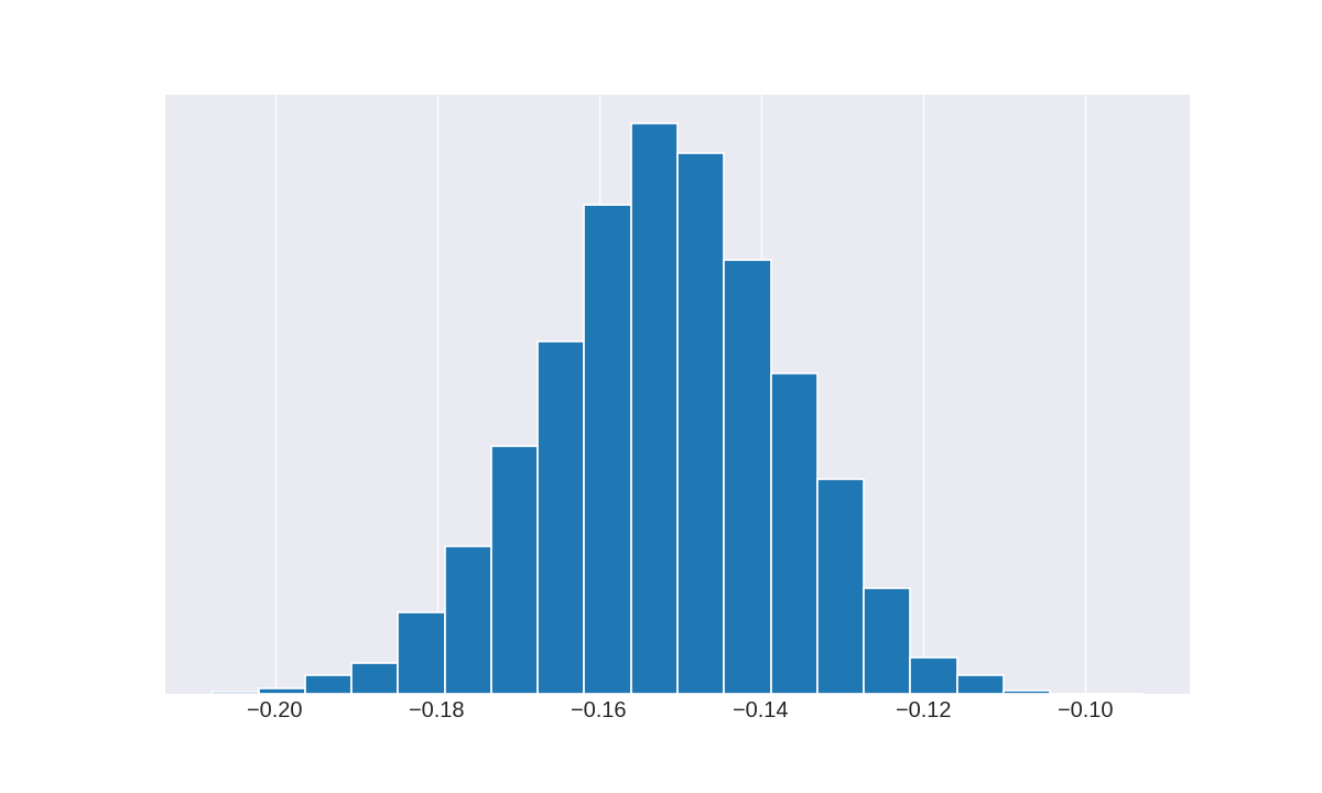
Do you know why that is weird?
The correct figure is (I think):

I have only changed the sign of res5. My Stan code could be wrong… but when you get the same figure with pymc3, you begin to doubt. The goal is then to improve the model (the diagnostics are not good), and that will be very hard.