Feedback on model for ecological inference

[William_Bradley]

I have been trying to model a basic ecological inference problem in RStan.

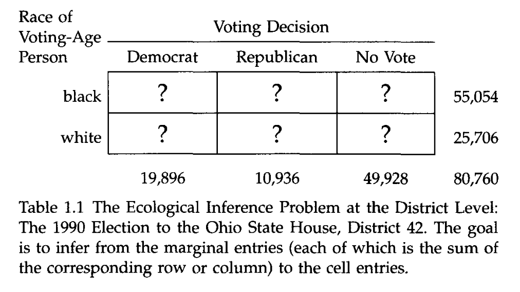
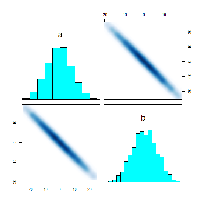
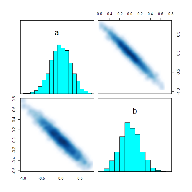
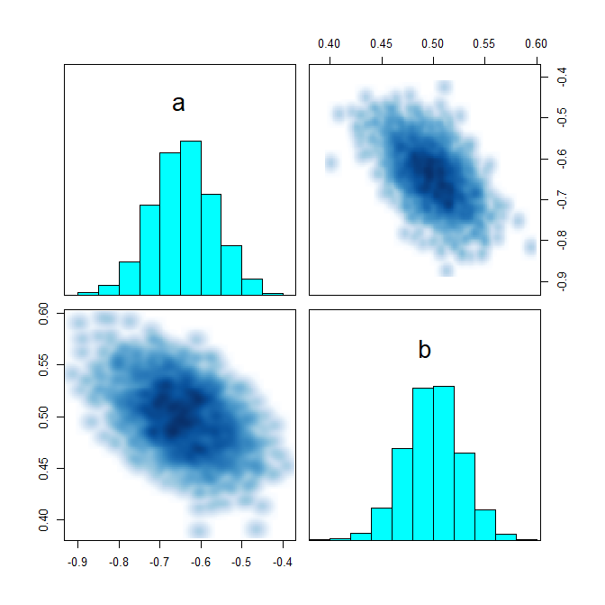
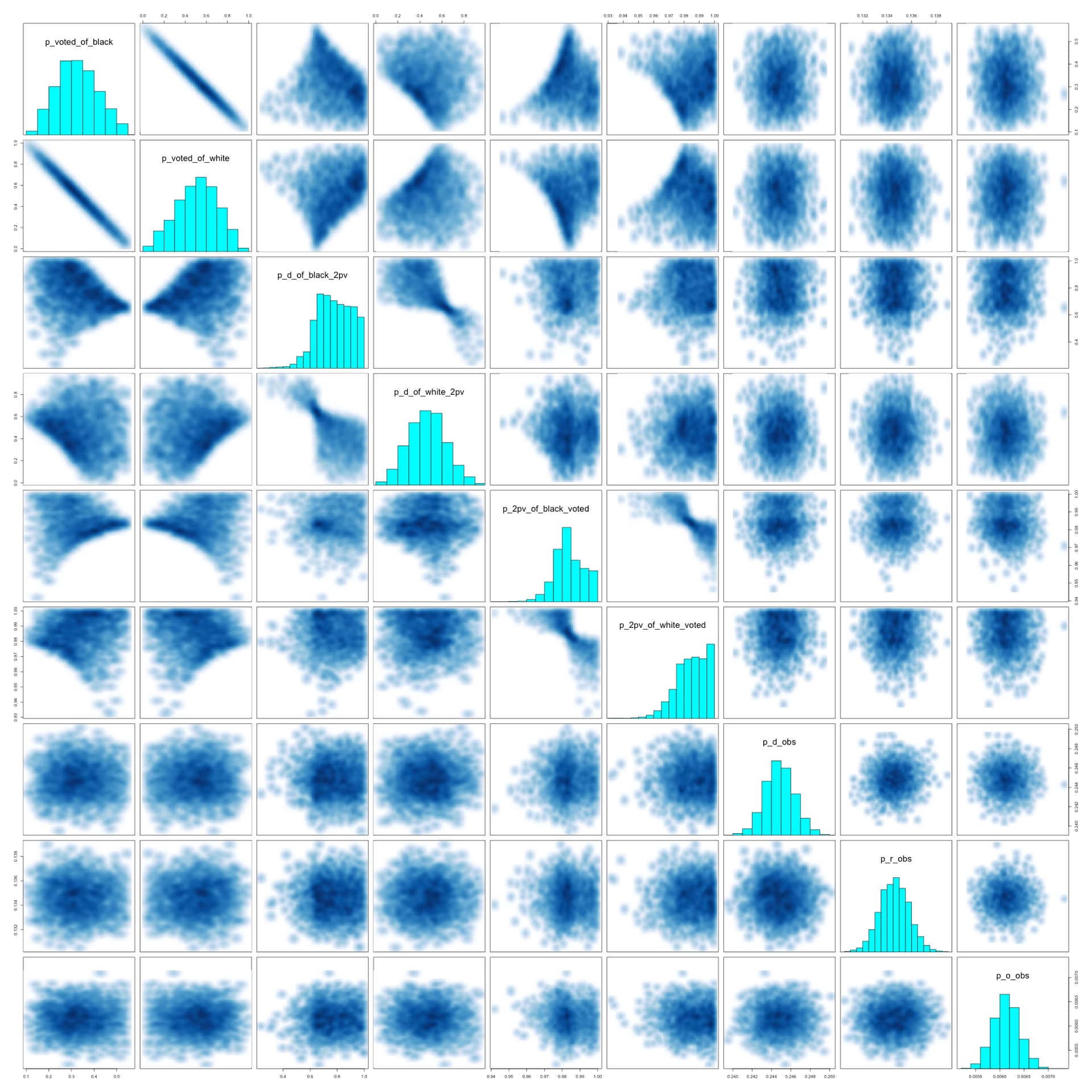
I have introduced a fourth column: third-party votes. I will make a hierarchical model that incorporates data from the precincts that partition the district, but I want to make sure I am doing everything right first. I believe this is a fairly nice parametrization, but I am new to Stan and I don’t really understand how to read the pairs() plots.

This is rstan version 2.32.7 (Stan version 2.32.2).

Results

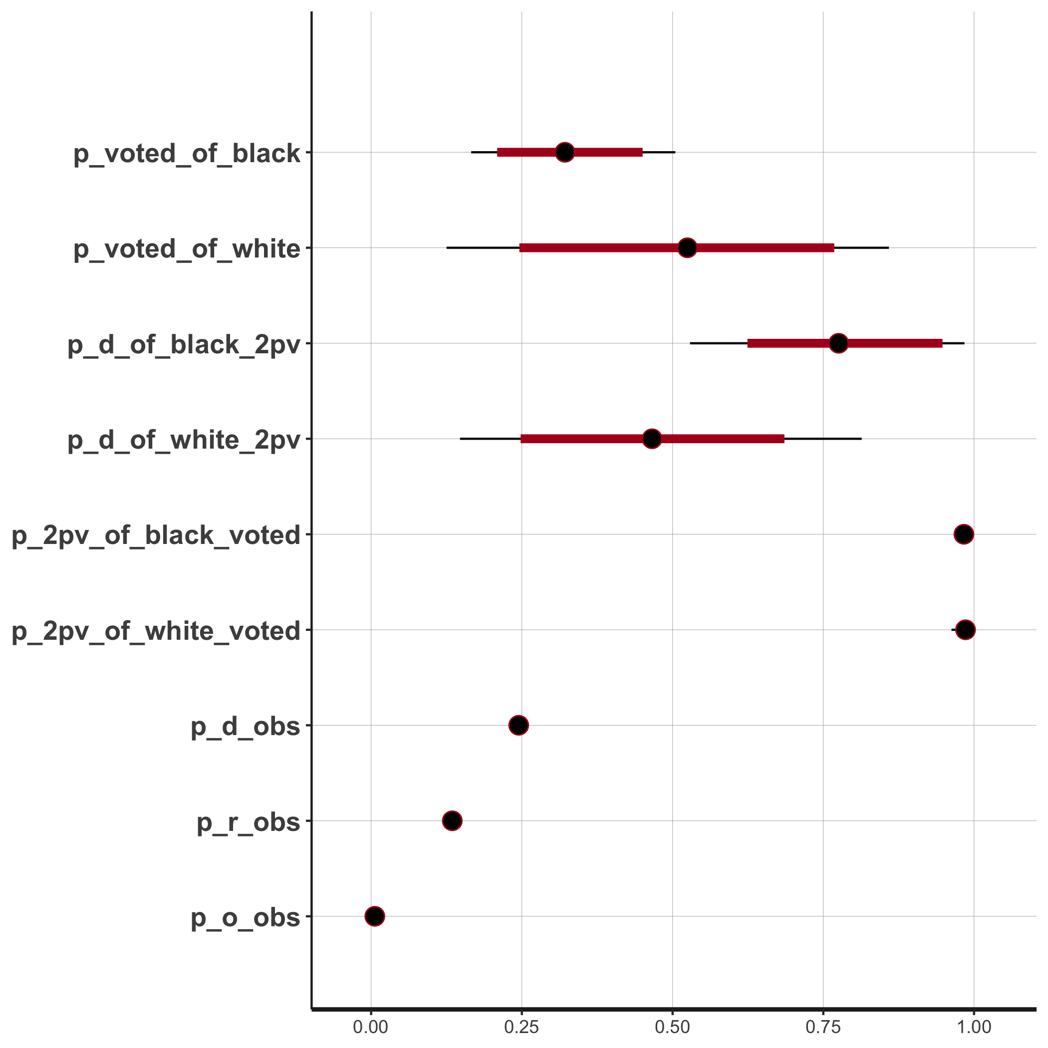
                     mean se_mean   sd 2.5%  25%  50%  75% 97.5% n_eff Rhat
p_voted_of_black     0.33    0.00 0.09 0.17 0.26 0.32 0.39  0.51  1168    1
p_voted_of_white     0.51    0.01 0.19 0.13 0.37 0.52 0.65  0.86  1165    1
p_d_of_black_2pv     0.78    0.00 0.13 0.53 0.68 0.78 0.88  0.98  1314    1
p_d_of_white_2pv     0.47    0.00 0.17 0.15 0.35 0.47 0.58  0.81  1538    1
p_2pv_of_black_voted 0.98    0.00 0.01 0.97 0.98 0.98 0.99  1.00  1650    1
p_2pv_of_white_voted 0.98    0.00 0.01 0.96 0.98 0.99 0.99  1.00  1626    1
p_d_obs              0.24    0.00 0.00 0.24 0.24 0.24 0.25  0.25  4382    1
p_r_obs              0.13    0.00 0.00 0.13 0.13 0.13 0.14  0.14  3762    1
p_o_obs              0.01    0.00 0.00 0.01 0.01 0.01 0.01  0.01  3866    1

(no warnings)

Stan code

data {
    int<lower=1> n; // total number of people in the district
    int<lower=0, upper=n> 
        d, r, o,  // Democratic votes, Republican votes, third-party votes (non-voters inferred)
        black;    // (white population inferred)
    // parameters for the (beta distribution) priors of 
    // P(voted|black), P(voted|white), 
    // P(D|black,voted D or R), P(D|white,voted D or R),
    // P(D or R|black,voted), P(D or R|white, voted)
    array[6] real<lower=0> alphas;
    array[6] real<lower=0> betas;
}
transformed data {
    real<lower=0, upper=1>
        p_black = (black + 0.0) / n,
        p_white = 1 - p_black;
}
parameters {
    real<lower=0, upper=1> 
        p_voted_of_black,     // P(voted|black)
        p_voted_of_white,     // P(voted|white)
        p_d_of_black_2pv,     // P(D|voted D or R,black)
        p_d_of_white_2pv,     // P(D|voted D or R,white)
        p_2pv_of_black_voted, // P(D or R|black,voted)
        p_2pv_of_white_voted; // P(D or R|white,voted)
}
transformed parameters {
    real<lower=0, upper=1> 
        p_d_obs,  // P(D) (estimated from parameters)
        p_r_obs,  // P(R) (estimated from parameters)
        p_o_obs;  // P(3rd party) (estimated from parameters)

    p_d_obs = p_d_of_black_2pv * p_2pv_of_black_voted * p_voted_of_black * p_black
            + p_d_of_white_2pv * p_2pv_of_white_voted * p_voted_of_white * p_white;
    p_r_obs = (1 - p_d_of_black_2pv) * p_2pv_of_black_voted * p_voted_of_black * p_black
            + (1 - p_d_of_white_2pv) * p_2pv_of_white_voted * p_voted_of_white * p_white;
    p_o_obs = (1 - p_2pv_of_black_voted) * p_voted_of_black * p_black
            + (1 - p_2pv_of_white_voted) * p_voted_of_white * p_white;
}
model {
    // Priors
    p_voted_of_black ~ beta(alphas[1], betas[1]);
    p_voted_of_white ~ beta(alphas[2], betas[2]);
    p_d_of_black_2pv ~ beta(alphas[3], betas[3]);
    p_d_of_white_2pv ~ beta(alphas[4], betas[4]);
    p_2pv_of_black_voted ~ beta(alphas[5], betas[6]);
    p_2pv_of_white_voted ~ beta(alphas[6], betas[6]);

    d ~ binomial(n, p_d_obs);
    r ~ binomial(n, p_r_obs);
    o ~ binomial(n, p_o_obs);
}

R code

# pp. 13 of King
library(rstan)
library(ggplot2)

seed <- 1
set.seed(seed)

o <- 500 # 3rd party votes
n <- 80760 + o
d <- 19896
r <- 10936
nv <- 49928
black <- 55054 + o
white <- 25706

stopifnot(d + r + o + nv == n, black + white == n)

prior_alphas <- c(2, 2, 4, 2.5, 100, 100)
prior_betas <- c(2, 2, 1, 2.5, 1, 1)

data <- list(n = n, d = d, r = r, o = o, black = black, alphas = prior_alphas, betas = prior_betas)

fit <- stan(
    file = "ohio-state-house-42.stan",
    data = data,
    chains = 4,
    warmup = 1000,
    iter = 2000,
    cores = 4,
    seed = seed
)

pars <- c("p_voted_of_black", "p_voted_of_white",
          "p_d_of_black_2pv", "p_d_of_white_2pv",
          "p_2pv_of_black_voted", "p_2pv_of_white_voted",
          "p_d_obs", "p_r_obs", "p_o_obs")

print(fit, pars = pars)
plot(fit, pars = pars)
ggsave("ohio-state-house-42.png")

png("ohio-state-house-42-pairs.png", height = 2000, width = 2000)
suppressWarnings(pairs(fit, pars = pars))
dev.off()

[jd_c]

Howdy!
I think you have a combination of additive and multiplicative degeneracies (see Identity Crisis ) that manifest as the strange shapes in your pairs plots. When I first saw this, I couldn’t believe that HMC didn’t complain, so I had to run it for myself to see (thanks for the code!)…perhaps because the parameters are bounded zero to one helps. Anyway, when you look at the very top left corner plot you can see that p_voted_of_black is strongly correlated to p_voted_of_white, which is not surprising, given that these are both parameters and they are added together (eventually added together after each being multiplied by constants and other parameters). This strong correlation is telling you that you can’t really learn much about the parameters individually but rather only the combination of the two them. Since these parameters with an additive degeneracy are then each multiplied by other parameters, I think you get the strange shapes with boundaries in the pairs plots - the result of combining additive and multiplicative degeneracies.
The usual solutions are adding more data that specifically inform individual parameters through another model (say a ‘joint’ model), giving up and combining parameters, or maybe really strong priors. In other words, to put it simply, either include more information or adjust your expectations of what can be inferred. However, given that you are trying to solve the problem in the table without more information, I’m not sure you have many options.

[William_Bradley]

Thank you! Would you mind explaining what a “joint” model means, as well as how I would combine parameters? I think there is actually more information I can add, i.e. precinct-level estimates via a hierarchical model.

Also, I’m fine with my inference being fairly uninformative (and I expected this), but is it wrong? I had assumed not because HMC converged without warnings.

[jd_c]

@William_Bradley

Would you mind explaining what a “joint” model means,

The use of the word might be sloppy terminology on my part, but this is what I was trying to convey: Since the main problem here is lack of information, you need to find some way to incorporate more information if you want to learn about these parameters individually. Right now, there are infinitely many combinations of your parameters that ‘work’ for your model. One way to provide more information would be if you had some sort of auxiliary data that specifically informed individual parameters. For example, suppose you had some survey data that informed p_voted_of_black and some other data that informed p_2pv_of_black_voted. You could include those two models and data in your above Stan code. This is described in section 3.1 and fleshed out in a simple example with Stan code in section 5.2 that I linked to above (and I give a simple example in m4 below). These models of auxiliary data that included those individual parameters would help infer them, subsequently constraining the parameters like p_voted_of_white that are currently correlated, to a narrow region.

@William_Bradley

as well as how I would combine parameters?

Say you have something like:

stan_model1 <- "
transformed data {
  vector[100] y;
    for (n in 1:100) {
      y[n] = normal_rng(0, 1);
    }
}
parameters {
  real a;
  real b;
}
model {
  a ~ normal(0, 10);
  b ~ normal(0, 10);
  y ~ normal(1.5*a + 2*b, 1);
}
"

m1 <- stan(model_code = stan_model1, chains = 4, cores = 4, seed=392709)

print(m1, pars=c("a","b"))

pairs(m1, pars=c("a","b"))

Notice that the parameters are strongly correlated and that they are constrained by the priors.
If we don’t have any additional information about a or b, then we should recognize that we can’t learn much about them individually but only their sum. So, we might adjust our expectations of what we can learn, and combine them into a single parameter c = 1.5*a + 2*b.

stan_model2 <- "
transformed data {
  vector[100] y;
    for (n in 1:100) {
      y[n] = normal_rng(0, 1);
    }
}
parameters {
  real c;
}
model {
  c ~ normal(0, 10);
  y ~ normal(c, 1);
}
"

m2 <- stan(model_code = stan_model2, chains = 4, cores = 4, seed=392709)

print(m2, pars=c("c"))

Inference on the parameter c is excellent.

Now, if we do have more information on a and b, it could come in a couple of forms. Suppose we have strong prior information on b but not a. We can incorporate that in the model to better infer both a and b.

stan_model3 <- "
transformed data {
  vector[100] y;
    for (n in 1:100) {
      y[n] = normal_rng(0, 1);
    }
}
parameters {
  real a;
  real b;
}
model {
  a ~ normal(0, 10);
  b ~ normal(0, 0.2);
  y ~ normal(1.5*a + 2*b, 1);
}
"

m3 <- stan(model_code = stan_model3, chains = 4, cores = 4, seed=392709)

print(m3, pars=c("a","b"))

pairs(m3, pars=c("a","b"))

We can see that although they are still strongly correlated, a is now constrained to a much narrower region (check the axis limits in this plot vs the one above for a), since we have given the model more information about b.

The other way we might have more information is if we had auxiliary data that informed b itself. We could include a model of the auxiliary data and b, which will allow us to better infer a as well.

stan_model4 <- "
transformed data {
  vector[100] y;
  vector[100] bx;
    for (n in 1:100) {
      y[n] = normal_rng(0, 1);
      bx[n] = normal_rng(0.5, 0.25);
    }
}
parameters {
  real a;
  real b;
  real<lower=0> sigma;
}
model {
  a ~ normal(0, 10);
  b ~ normal(0, 10);
  sigma ~ normal(0, 1);
  bx ~ normal(b, sigma);
  y ~ normal(1.5*a + 2*b, 1);
}
"

m4 <- stan(model_code = stan_model4, chains = 4, cores = 4, seed=392709)

print(m4, pars=c("a","b","sigma"))

pairs(m4, pars=c("a","b"))

While there is perhaps still a mild correlation, inference is much better for both a and b and the correlation between the two is much weaker.

@William_Bradley

Also, I’m fine with my inference being fairly uninformative (and I expected this), but is it wrong? I had assumed not because HMC converged without warnings.

I suppose that depends on how one defines “wrong”. HMC does its job without complaint in your case above (with the seed that you chose), and if you program a generated quantities section for your model to predict d, r, and o, there is no tension between histograms of predictions and the values of d, r, and o (I did this yesterday but trashed the code). It makes decent predictions. However, what have you learned? Not really anything about the individual parameters beyond the prior information that you put in to the model.

For example, let’s take the degenerate m1 example model above and add a generated quantities section to check summaries of our model predictions vs the same summaries of observations. For easier plotting I use Betancourt’s tools here mcmc_visualization_tools/r at main · betanalpha/mcmc_visualization_tools · GitHub

stan_model1b <- "
transformed data {
  vector[100] y;
    for (n in 1:100) {
      y[n] = normal_rng(0, 1);
    }
}
parameters {
  real a;
  real b;
}
model {
  a ~ normal(0, 10);
  b ~ normal(0, 10);
  y ~ normal(1.5*a + 2*b, 1);
}
generated quantities {
  vector[100] y_pred;
  vector[100] y_obs = y;
    for (n in 1:100) {
      y_pred[n] = normal_rng(1.5*a + 2*b, 1);
    }
}
"

m1b <- stan(model_code = stan_model1b, chains = 4, cores = 4, seed=392709)

util <- new.env()
source('mcmc_analysis_tools_rstan.R', local=util)
source('mcmc_visualization_tools.R', local=util)

samples1 <- util$extract_expectand_vals(m1b)
y <- extract(m1b)$y
y_obs <- extract(m1b)$y_obs

util$plot_hist_quantiles(samples1, 'y_pred', -5, 5, 0.5, baseline_values=y_obs[1,1:100], xlab="y values")

There’s little tension between the summaries (histogram) of predictions and the summaries (histogram) of observations, even though the model is degenerate. It makes fine predictions. But that doesn’t mean we actually learned anything about our individual parameters a and b.