I feel this is a classical textbook example, but I can’t find it. Here is some fake data where some continuous variable y is measured over some geographical gradient (a continuous predictor x). Three species were measured for y at each of 5 sites (i.e., species and site are crossed factors). The data plots as following:
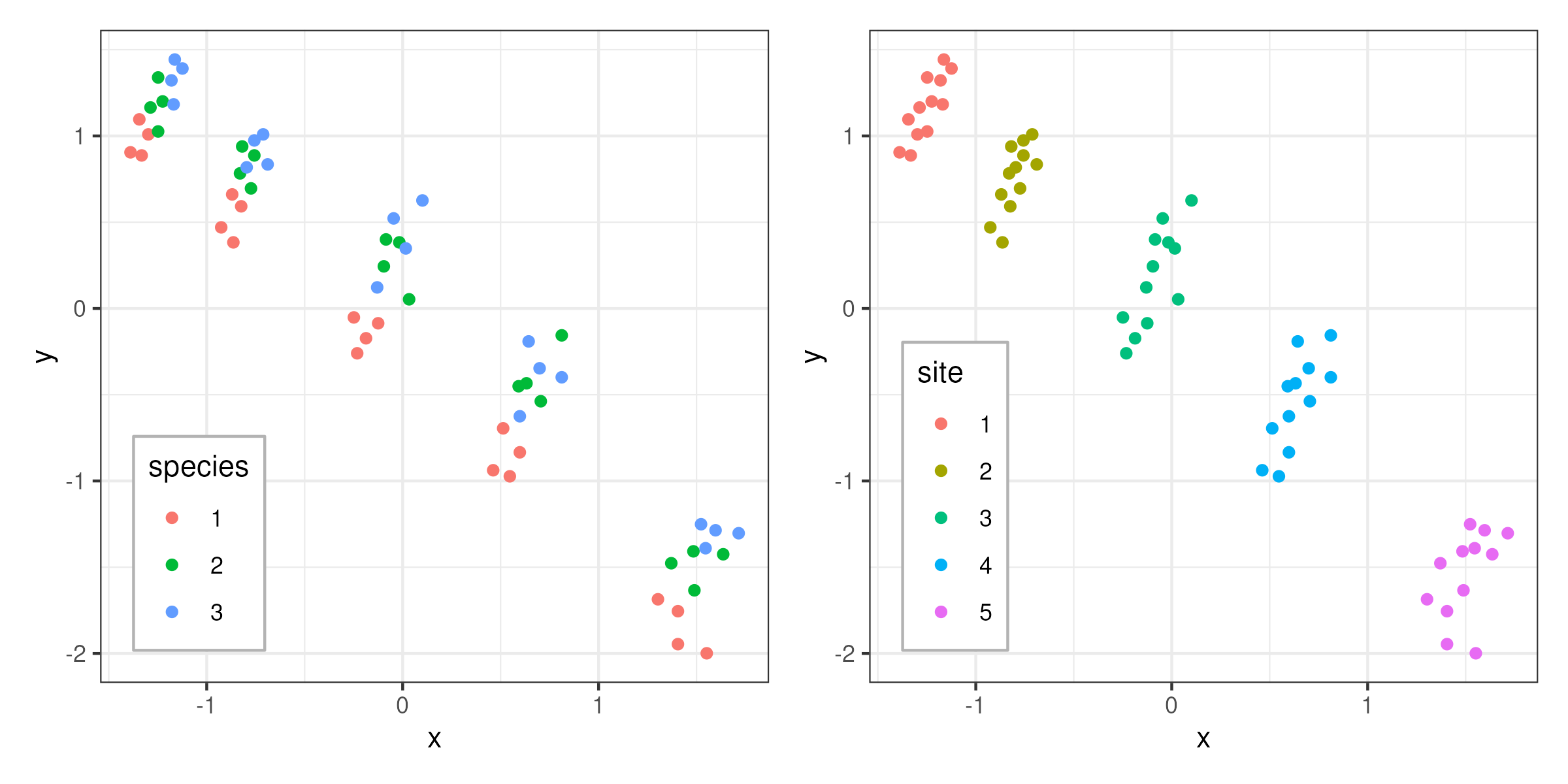
Let’s say we want to fit a linear model of y against x and let the intercept vary with species. I am trying to figure out how to account for the fact measurements come from sites. I have tried to add a varying intercept for each site but this alters the fixed slope so I am a bit confused and suspect my approach is wrong.
Find below what I have implemented so far.
Math notation with one varying intercept (m1):
Math notation with two varying intercepts (m2):
Stan model with one varying intercept (m1):
data {
  int<lower=0> N;
  int<lower=0> N_species;
  array[N] int<lower=1> species;
  vector[N] y;
  vector[N] x;
}

parameters {
  real alpha_bar;
  vector[N_species] alpha1;
  real beta;
  real<lower=0> sigma_alpha1;
  real<lower=0> sigma;
}

model {

  // hyper-priors
  target += std_normal_lpdf(alpha_bar); // same as normal_lpdf(alpha_bar | 0, 1)
  target += std_normal_lpdf(beta); // same as normal_lpdf(beta | 0, 1)
  target += exponential_lpdf(sigma_alpha1 | 1);
  target += exponential_lpdf(sigma | 1);

  // adaptive priors
  target += normal_lpdf(alpha1 | alpha_bar, sigma_alpha1);

  //likelihood
  target += normal_lpdf(y | alpha1[species] + beta * x, sigma);

}
Stan model with two varying intercepts (m2):
data {
  int<lower=0> N;
  int<lower=0> N_sites;
  int<lower=0> N_species;
  array[N] int<lower=1> site;
  array[N] int<lower=1> species;
  vector[N] y;
  vector[N] x;
}

parameters {
  real alpha_bar;
  vector[N_species] alpha1;
  vector[N_sites] alpha2;
  real beta;
  real<lower=0> sigma_alpha1;
  real<lower=0> sigma_alpha2;
  real<lower=0> sigma;
}

model {

  // hyper-priors
  target += std_normal_lpdf(alpha_bar); // same as normal_lpdf(alpha_bar | 0, 1)
  target += std_normal_lpdf(beta); // same as normal_lpdf(beta | 0, 1)
  target += exponential_lpdf(sigma_alpha1 | 1);
  target += exponential_lpdf(sigma_alpha2 | 1);
  target += exponential_lpdf(sigma | 1);

  // adaptive priors
  target += normal_lpdf(alpha1 | alpha_bar, sigma_alpha1);
  target += normal_lpdf(alpha2 | 0, sigma_alpha2);

  //likelihood
  target += normal_lpdf(y | alpha1[species] + alpha2[site] + beta * x, sigma);

}
Fake data:
site <- c(1, 1, 1, 1, 2, 2, 2, 2, 3, 3, 3, 3, 4, 4, 4, 4, 5, 5, 5, 5, 1, 1, 1, 1, 2, 2, 2, 2, 3, 3, 3, 3, 4, 4, 4, 4, 5, 5, 5, 5, 1, 1, 1, 1, 2, 2, 2, 2, 3, 3, 3, 3, 4, 4, 4, 4, 5, 5, 5, 5)
species <- c(1, 1, 1, 1, 1, 1, 1, 1, 1, 1, 1, 1, 1, 1, 1, 1, 1, 1, 1, 1, 2, 2, 2, 2, 2, 2, 2, 2, 2, 2, 2, 2, 2, 2, 2, 2, 2, 2, 2, 2, 3, 3, 3, 3, 3, 3, 3, 3, 3, 3, 3, 3, 3, 3, 3, 3, 3, 3, 3, 3)
x <- c(-1.389, -1.344, -1.332, -1.298, -0.926, -0.870, -0.864, -0.824, -0.232, -0.125, -0.249, -0.187, 0.547, 0.513, 0.462, 0.598, 1.552, 1.405, 1.303, 1.405, -1.287, -1.248, -1.225, -1.248, -0.830, -0.774, -0.757, -0.819, 0.033, -0.096, -0.085, -0.017, 0.592, 0.812, 0.632, 0.705, 1.489, 1.371, 1.484, 1.636, -1.180, -1.169, -1.124, -1.163, -0.757, -0.796, -0.689, -0.712, -0.130, 0.016, 0.101, -0.046, 0.598, 0.643, 0.699, 0.812, 1.523, 1.546, 1.597, 1.715)
y <- c(0.905, 1.096, 0.887, 1.009, 0.470, 0.661, 0.383, 0.592, -0.260, -0.086, -0.052, -0.173, -0.973, -0.695, -0.938, -0.834, -1.999, -1.755, -1.686, -1.946, 1.165, 1.026, 1.200, 1.339, 0.783, 0.696, 0.887, 0.939, 0.053, 0.244, 0.400, 0.383, -0.451, -0.156, -0.434, -0.538, -1.634, -1.477, -1.408, -1.425, 1.322, 1.183, 1.391, 1.443, 0.974, 0.818, 0.835, 1.009, 0.122, 0.348, 0.626, 0.522, -0.625, -0.191, -0.347, -0.399, -1.251, -1.390, -1.286, -1.303)
Fit models with cmdstanr:
library(cmdstanr)

## data list for Stan
dlist <- list(
  N = length(y),
  N_species = length(unique(species)),
  N_sites = length(unique(site)),
  species = species,
  site = site,
  x = x,
  y = y
)

## compile models
m1 <- cmdstan_model("mod1.stan")
m2 <- cmdstan_model("mod2.stan")

## fit models
fit1 <- m1$sample(data = dlist, chains = 4, parallel_chains = 4, refresh = 1000, seed = 123)
fit2 <- m2$sample(data = dlist, chains = 4, parallel_chains = 4, refresh = 1000, seed = 123)
Resulting slopes
> fit1$summary("beta")
# A tibble: 1 × 10
  variable   mean median     sd    mad    q5    q95  rhat ess_bulk ess_tail
  <chr>     <num>  <num>  <num>  <num> <num>  <num> <num>    <num>    <num>
1 beta     -0.967 -0.967 0.0226 0.0216 -1.00 -0.930  1.00    3891.    2356.
> fit2$summary("beta")
# A tibble: 1 × 10
  variable   mean median    sd   mad     q5   q95  rhat ess_bulk ess_tail
  <chr>     <num>  <num> <num> <num>  <num> <num> <num>    <num>    <num>
1 beta     0.0916  0.138 0.375 0.330 -0.706 0.608  1.00     625.     289.