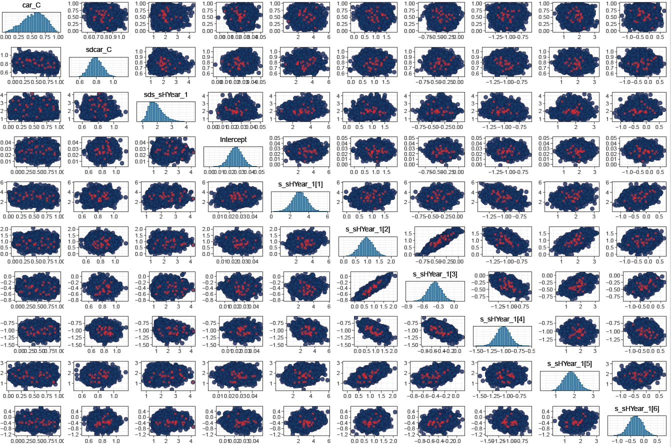
Hey! I am quite new in Stan and I would like to know what this photo produced by shinystan tells me about my divergent transitions. I had 25 divergent transitions and would like to know whether they are something serious.
They seem to be randomly scattered around the bulk of the density in all plots
EDIT: I’ll add info that my data has some big outliers, so could those result in these divergent transitions?
Yes, they are something serious. It’s a sensitive signal, but 25 is not likely to be a false positive for problems with sampling.
The plot doesn’t say that much about what may be causing these divergences, other than how they are distributed within the distribution of the log posterior probability of the fit.
A pairs plot with divergences marked would be more helpful. Perhaps also some more details about your data and model?
You mention outliers - do you model these in any way? What are they likely to represent?
I’ll come back with pair plots, but first quick reply. I have quite few parameters because I have a distributional model with location and scale parameters. I also have one hierarchical spatial effect, which produces quite many parameters. However, I did get divergences before including the spatial effect.
My data is log-normally distributed, so I am modelling log-rates. Because rates are calculated from two observations, the likely reason for such a high rates (outliers) is that one of the two observations is faulty. This can happen at the spatial edges of the phenomenon, where the observations have small values and are suspect to random changes. Can also be due to observational error. Like, if the rate is 100/10, that is likely unnatural.
This is modelled with the scale parameters, I am modelling the increase in variance with decrease in observed values. So if the rate is calculated from small observed value, then it is likely to have higher variance than if it were calculated from bigger values.
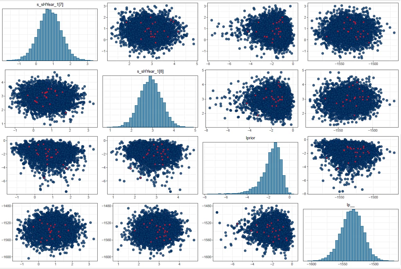
Your plots show the density of the log-posterior values themselves without any reference to parameter values. A more useful, but still limited, visualization in 2D (in practice a 3D graph flattened into 2D as a sort of heatmap) would be the density of the log posterior as a function of a pair of variables (e.g. this one). That would give you a sense of where in parameter space divergent transitions are coming up more frequently.
It may be that the distributions are not actually that different, just that you have few data points for the divergent transitions (not sure how your violin plots display outliers).
Hm. Not immediately obvious to me what it might be, but the strong posterior correlation between ssHyear1 2 & 3 would be a suspect.
EDIT: Your post strengthens that suspicion, then. Do you know anything about your data that might induce a positive correlation between these two? I’m not so familiar with the parametrization behind s().
Those parameters are tricky because they are the basis coefficients of the smooth function. I can only influence those parameters via the sds_sHYear parameter.
I did notice that when I changed my prior from half_normal(0, 2) to half_normal(0, 3), the number of divergent transitions increased to over 60. These parameters are hard to interpret, the sds_HYear parameter defines how much these individual s_sHYear parameters vary.
I’ll attempt two solutions next:
Change the maximum number of basis coefficients via k setting in the s()
Make the sds prior stricter (e.g. half-normal(0,1). However, I am not so confident in explaining this prior.
Decreasing the number of basis coefficients increased divergent transitions to over 900.
Making the SDS prior stricter (half-normal(0, 1) reduced the number of divergent transitions to 7, so I increased adapt_delta to 0.9 and it then got rid of the rest.
Yes, but divergences are a consequence of approximating continuous Hamiltonian dynamics on a high-dimensional parameter space, and the curvature that is problematic for the integrator (e.g. leapfrog) may happen in whatever number of those dimensions (and even if it is just a few or we can visualize it somehow it may not be easily identifiable).
functions that are very flexible, especially within other models can cause problems of identifiability and potentially divergences, but on the other hand they may be needed to fit the data. But apparently you were able to find the combination that would make ti work with respect to the divergences.