Sorry this is such a long post, but it was hard to give enough context to understand my problem and still be brief :-\
[first, context on my model]
I’ve been working for a while on fitting a model from neutrino physics to simulated data for a specific experiment. Fundamentally, the model has 3 parameters of interest, called \Delta m^2, \theta, and \delta; the latter two are angles and are therefore cyclic. The first one has no physical boundaries and all values are allowed. There are also numerous nuisance parameters that arise from the various systematic uncertainties in the simulation of the experiment, which are treated as Gaussian in this model.
The experiment has two detectors: one that is sensitive to both the parameters of interest and the nuisance parameters (let’s call it the “Physics Detector” for the purpose of this discussion); and a second detector which is sensitive only to a subset of the nuisance parameters, which is intended to constrain them (the “Systematics Detector”).
Because the simulation is run by an external library, I can’t use the Stan modeling language to fit it. But by reverse-engineering the code that comes out of CmdStan I’ve managed to figure out how to hook Stan up to the C++ interface of the code that drives the simulation. (I can give more details if needed.)
The likelihood given to Stan is computed by comparing histograms of measurements using a Poisson-inspired binned likelihood function; the simulation produces alternate histograms depending on the values of the physics & nuisance parameters.
[Ok, now my issue]
I’ve been exercising the model by fitting sets of simulated data using NUTS with a diagonal metric. Stan fits this model beautifully, and always converges to the correct answers, when I only fit the predictions for the Physics Detector, regardless of how many of the parameters of interest or nuisance parameters are included. It also fits the nuisance parameters successfully if I only fit the Systematics Detector alone. But when I attempt to fit the two together, Stan is in general unable to find the correct typical set for the parameters of interest; however, the nuisance parameters are correctly inferred. The values inferred for \Delta m^2 in particular are often orders of magnitude away from the correct answer.
I think this is because the curvature of the likelihood function in the nuisance directions is very different from that in the directions of the physics parameters. (That is, because the Systematics Detector constrains the nuisance parameters powerfully, the effect on the likelihood of changing the nuisance parameters is much stronger than changing the physics parameters.) I guess the ‘phase change’ in LL when the typical set around the nuisance parameters is found is somehow confusing the adaptation from continuing to converge onto the physics parameters?
By looking at the values chosen as a function of sample number during warmup, I see things that suggest this. (For the plots of parameters, correct values, where they are within the axis ranges, are given by the dotted lines.)
First, the (negative of) the log of the log likelihood (because so many orders of magnitude are being crossed; plotting LL makes it impossible to see any features):

Then the parameters of interest:


Lastly, the 5 nuisance parameters that were sampled in this particular run (I’ve done many others with anything from 1 to the whole suite of about 75, with similar results):


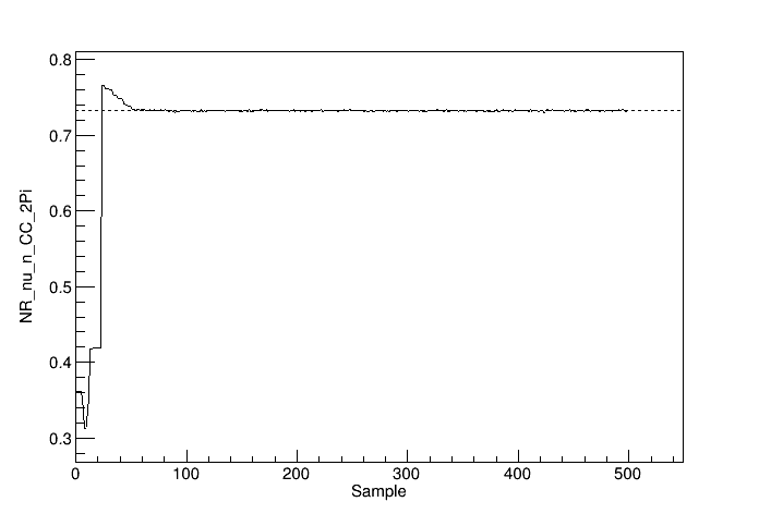

You can see Stan converging onto the correct values of the nuisance parameters in stages by sample 100 or so. Interestingly, two of the physics parameters hardly move at all until this, while \Delta m^2 moves at the beginning, but in the wrong direction (the correct value is +2.5). (I ran several hundred chains with the same settings and this behavior is fairly typical. Only about 15% of the chains even came close to the right neighborhood.)
I think it’s likely that the complexity of the model is part of the problem. E.g., if I brute-force scan across \Delta m^2 (with the other parameters held fixed at their correct values), the LL has a lot of features (note right plot is a zoom of the left with the correct value indicated by the pink arrow, the only point that’s actually at LL = 0):


It’s essentially a monotonic function on either side of the maximum (increasing below it, decreasing above it) convolved with two different periods of wiggles. It seems that Stan is usually getting stuck in one of the larger period wiggles. What baffles me, though is that (as noted above) Stan has no trouble fitting this model and finding the maximum when I don’t include the second detector constraint (even if the same nuisance degrees of freedom are incorporated).
I’ve tried numerous iterations on this to see if I can get the exploration of the physics parameter space to improve (with several hundred chains in each permutation to make sure it wasn’t a function of the initialization point):
- Increasing the number of warmup samples (though from these metrics you can see it’s probably fully warmed up by around sample 100, and that’s also typical)
- Increasing the number of samples used in the initial “fast” adaptation period (
init_buffer = 125in CmdStan parlance) - Varying
adapt_delta: tried 0.85, 0.9, 0.95 with only marginal improvements
I don’t quite understand the adaptation process well enough to be able to guess whether I should keep trying more values for these hyperparameters (adapt_delta=0.99?) or whether there are other things I should try instead (use a dense mass matrix?).
Does anyone have advice on what I can try to help Stan explore the model space better?
I’m more than happy to supply any other plots or further info if that would be helpful to try to figure out what’s going on. (There’s also no reason I couldn’t share the code, though it’s bolted onto a much larger framework that is unlikely to give a non-expert much insight without weeks of study, so I’m not inclined to go that route unless somebody wants to work on this longer-term with me.)
I’d love any insight anyone can offer!