Using {projpred} latent projection with {brms} Weibull family models

[rtnliqry]

@fweber144

Yes, this is what I meant with … However, as noted above, this more general (and hence more desirable) solution is probably more tedious to implement.

Got you, sorry, I was slow to realise this!

@avehtari

Now I think we need to sample the missing censored observations from a truncated Weibull with the left truncation at the censoring time. Given the augmented observations, we can then use just the latent of Weibull (we can’t mix latent of Weibull and latent of Bernoulli).

@avehtari Did you have any thoughts on this?

[avehtari]

@rtnliqry

@avehtari Did you have any thoughts on this?

I’ve been on vacation, and now slowly going through the pile of emails. I have not thought further about this during my vacation, but I still think this is the way to do it.

[fweber144]

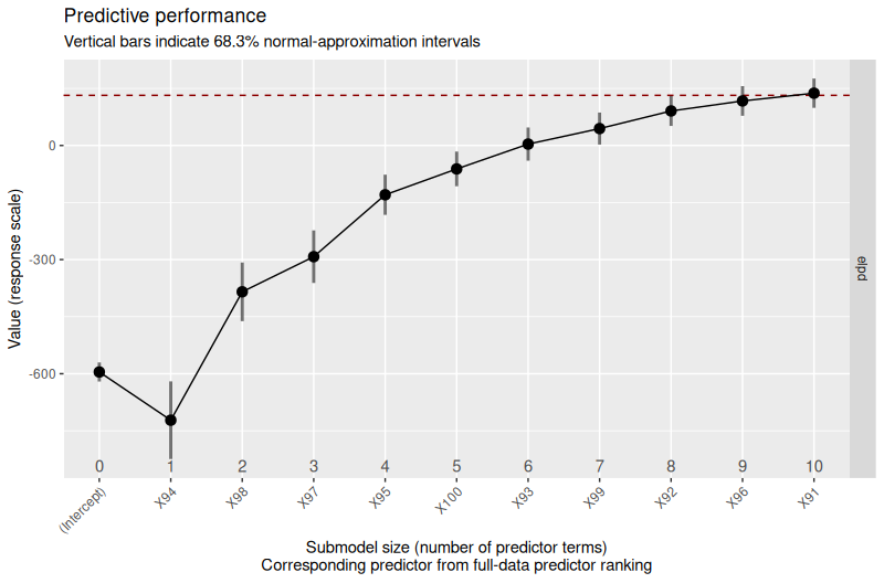
I have implemented a draft solution for this in #528. Here is the updated Weibull example from above which illustrates this (plots are shown below):

## Packages ----

library(brms)
library(MASS)
library(Matrix)
### Installed from <https://github.com/fweber144/projpred/tree/cens_latent>, the
### branch for PR [#528](https://github.com/stan-dev/projpred/pull/528):
library(projpred)
###
# library(trialr)

## Simulate data ----

set.seed(1234)

### Deactivated to avoid package 'trialr':
# # Sample from LKJ distribution for a randomised correlation matrix
# cor_mat <- trialr::rlkjcorr(n = 1, K = 100, eta = 1)
###
cor_mat <- matrix(0, nrow = 100, ncol = 100)

# First and second variable sets correlate with each another within each set
cor_mat[91:95, 91:95] <- matrix(rep(0.5, times = 25), ncol = 5)
cor_mat[96:100, 96:100] <- matrix(rep(0.5, times = 25), ncol = 5)

# First and second variable sets do not correlate with one another between sets
cor_mat[91:95, 96:100] <- matrix(rep(0, times = 25))
cor_mat[96:100, 91:95] <- matrix(rep(0, times = 25))
diag(cor_mat) <- 1

# Sample some standard deviations of the variables
sd <- rgamma(100, 1, 2)

# Convert the correlation matrix to a covariance matrix
cov_mat <- diag(sd) %*% cor_mat %*% diag(sd)

# number of observations
n_obs <- 500

# Sample variables from the multivariate normal distribution
vars <- MASS::mvrnorm(
  n = n_obs
  ,mu = rnorm(100, 30, 2.5)
  ,Sigma = Matrix::nearPD(cov_mat)$mat
)

# Scale the variables
scaled_vars <- apply(vars, 2, scale, scale = TRUE)

# Draws from Weibull distribution where only the last set of variables have predictive information
shape <- 1.2
predictors <- scaled_vars[,91:100] %*% rep(c(0.5, -0.5), each = 5)
linpred <- exp(0 + predictors)
scale_pred <- linpred / (gamma(1 + (1 / shape))) # brms AFT parameterisation

y <- rweibull(
  n = n_obs
  ,shape = shape
  ,scale = scale_pred
)

cens <- runif(n_obs, 0, 4)
time <- pmin(y, cens)
status <- as.numeric(y <= cens)

df_sim <- data.frame(
  time = time
  ,censored = 1 - status
  ,vars
)

## Fit model using 'brms' ----

# Ignore a few divergent transitions for now:
model_hs <- brm(
  time | cens(censored) ~ 1 + .
  ,family = weibull
  ,data = df_sim
  ,prior = c(
    prior(normal(0, 100), class = Intercept)
    ,prior(horseshoe(par_ratio = 0.1), class = b)
    ,prior(gamma(1, 0.5), class = shape)
  )
  ,seed = 1234
  ,chains = 4
  ,cores = 4
  ,control = list(adapt_delta = 0.95, max_treedepth = 15)
  ,save_pars = save_pars(all = TRUE)
)

## projpred ----

### Custom extend_family() functions ----
### for Weibull family latent projection as per
### <https://mc-stan.org/projpred/articles/latent.html#negbinex>

# Needed for these custom extend_family() functions:
refm_shape <- as.matrix(model_hs)[, "shape", drop = FALSE]

### Not necessary (projpred's internal default for `latent_ilink` works
### correctly in this case):
# latent_ilink_weib <- function(
    #     lpreds
#     ,cl_ref
#     ,wdraws_ref = rep(1, length(cl_ref))
# ) {
#
#   ilpreds <- exp(lpreds) # mu parameter link = "log"
#   return(ilpreds)
#
# }
###

latent_ll_oscale_weib <- structure(function(
    ilpreds,
    dis = rep(NA, nrow(ilpreds)),
    y_oscale,
    wobs = rep(1, ncol(ilpreds)),
    cens,
    cl_ref,
    wdraws_ref = rep(1, length(cl_ref))
) {
  idxs_cens <- which(cens == 1)
  idxs_event <- setdiff(seq_along(cens), idxs_cens)
  wobs_mat <- matrix(wobs, nrow = nrow(ilpreds), ncol = ncol(ilpreds),
                     byrow = TRUE)
  refm_shape_agg <- cl_agg(refm_shape, cl = cl_ref, wdraws = wdraws_ref)
  ll_unw <- matrix(nrow = nrow(ilpreds), ncol = ncol(ilpreds))
  for (idx_cens in idxs_cens) {
    ll_unw[, idx_cens] <- pweibull(
      y_oscale[idx_cens],
      shape = refm_shape_agg,
      scale = ilpreds[, idx_cens] / gamma(1 + 1 / as.vector(refm_shape_agg)),
      lower.tail = FALSE,
      log.p = TRUE
    )
  }
  for (idx_event in idxs_event) {
    ll_unw[, idx_event] <- dweibull(
      y_oscale[idx_event],
      shape = refm_shape_agg,
      scale = ilpreds[, idx_event] / gamma(1 + 1 / as.vector(refm_shape_agg)),
      log = TRUE
    )
  }
  return(wobs_mat * ll_unw)
}, cens_var = ~ censored)

latent_ppd_oscale_weib <- function(
    ilpreds_resamp,
    dis_resamp = rep(NA, nrow(ilpreds_resamp)),
    wobs = rep(1, ncol(ilpreds_resamp)),
    cl_ref,
    wdraws_ref = rep(1, length(cl_ref)),
    idxs_prjdraws
) {
  warning("The draws from this `latent_ppd_oscale` function are uncensored.")
  refm_shape_agg <- cl_agg(refm_shape, cl = cl_ref, wdraws = wdraws_ref)
  refm_shape_agg_resamp <- refm_shape_agg[idxs_prjdraws, , drop = FALSE]
  ppd <- rweibull(
    prod(dim(ilpreds_resamp)),
    shape = refm_shape_agg_resamp,
    scale = ilpreds_resamp / gamma(1 + 1 / as.vector(refm_shape_agg_resamp))
  )
  ppd <- matrix(ppd, nrow = nrow(ilpreds_resamp), ncol = ncol(ilpreds_resamp))
  return(ppd)
}

### Reference model object for latent projection ----

refm_hs_weib <- get_refmodel(
  model_hs
  ,latent = TRUE
  # ,latent_ilink = latent_ilink_weib
  ,latent_ll_oscale = latent_ll_oscale_weib
  ,latent_ppd_oscale = latent_ppd_oscale_weib
)

### Variable selection ----

### For setting `parallel = TRUE` in cv_varsel() (requires
### `validate_search = TRUE`):
# ncores_cv <- 7 # change this if necessary
# doParallel::registerDoParallel(ncores_cv)
# options(projpred.export_to_workers = c("refm_shape"))
###

# For simplicity (ignoring some bad Pareto k-values for now):
refm_hs_weib_vsel_loo_valsearchF <- cv_varsel(
  refm_hs_weib
  ,method = "forward"
  ,cv_method = "LOO"
  ,seed = 1234
  ,validate_search = FALSE # purely for speed
  ,nterms_max = 10
)

plot(refm_hs_weib_vsel_loo_valsearchF)

### If running the CV in parallel:
# # Tear down the CV parallelization setup:
# doParallel::stopImplicitCluster()
# foreach::registerDoSEQ()
###

### Final projection ----

prj <- project(
  refm_hs_weib,
  predictor_terms = paste0("X", 91:100)
)

### Prediction ----

prj_predict <- proj_predict(prj, .seed = 6230)
# Using the 'bayesplot' package:
library(bayesplot)
bayesplot_theme_set(ggplot2::theme_bw())
ppc_km_overlay(y = df_sim$time, yrep = prj_predict,
               status_y = 1 - df_sim$censored)

The predictive performance plot produced by this code looks as follows:

Hence, the truly relevant predictors are identified correctly (I increased the number of observations to 500 here to reduce noise from the observation model; a better way would be a simulation study of course).

The bayesplot::ppc_km_overlay() plot produced by this code looks as follows:

As you can see (by comparing this code to the code from Using {projpred} latent projection with {brms} Weibull family models - #15 by rtnliqry), I decided not to introduce any censoring-specific modification to the latent_ppd_oscale function. The reason is that the uncensored predictive distribution may already be enough (e.g., bayesplot::ppc_km_overlay() may be used for a “posterior-projection predictive check”, as illustrated here). If you really need censoring-specific modifications in the latent_ppd_oscale function, let me know.

Perhaps I’ll also add a log-normal example, but I have to see when I get the time for this.

[rtnliqry]

Thanks, both, for your continued input!

@avehtari

Now I think we need to sample the missing censored observations from a truncated Weibull with the left truncation at the censoring time. Given the augmented observations, we can then use just the latent of Weibull (we can’t mix latent of Weibull and latent of Bernoulli).

Just to make sure my understanding is correct: is integrating out the censored observations in latent_ll_oscale with pweibull equivalent to what you were suggesting, @avehtari? Or was the idea to create “pseudo”-observations for the censored observations by using rweibull (left-truncated at the known censored time), and then using dweibull on these augmented times?

@fweber144

As you can see (by comparing this code to the code from Using {projpred} latent projection with {brms} Weibull family models - #15 by rtnliqry), I decided not to introduce any censoring-specific modification to the latent_ppd_oscale function.

Yes, to be honest, I wasn’t really sure whether censoring the PPD was necessary. Presumably, by taking the censoring into account in fitting the reference model and in latent_ll_oscale, the PPD captures the uncertainty introduced by the censored observations anyway? Given that the censoring process is assumed to be random/independent of the outcome/predictors, I suppose one could at least censor predicted times that are greater than the last observed uncensored event time?

@fweber144

Perhaps I’ll also add a log-normal example, but I have to see when I get the time for this.

Thank you! I’m hoping the log-normal should be fairly straightforward for me to implement, assuming substituting pweibull and dweibull for plnorm and dlnorm into latent_ll_oscale as per the code above will be appropriate?