Understanding reparameterization of nonlinear hierarchical models with brms

I have a few questions about the brms parameterisation, and about how one might go about reparameterising a model with brms.

I’m working on trying to improve performance of a model that I’m working with to avoid funnel geometry of my posterior. I’ve been working through Michael Betancourt’s case study on hierarchical models to understand this better, and learning how, depending on whether the likelihood is minimally or maximally informative, a non-centred or centred parameterisation is optimal (NCP and CP). I’m just having some difficulty understanding the brms parameterisation.

Here I’ve used a toy example model based on another example that I found elsewhere in the forums, where the data is a built-in dataset. But it replicates the behaviour that I’m struggling with in my main model, which is more complicated.

data("Orange")	

dat1 <- data.frame(t = Orange$age, 	
                   y = Orange$circumference, 	
                   group = Orange$Tree)	

So, from this post (Disable non-centered parameterization in brms - #7 by paul.buerkner) (and from the brms documentation), I understand that brms, by default, makes use of NCP for nonlinear parameters, and did not previously allow a CP. However, from this more recent post (Non-centered population-level intercept - #5 by paul.buerkner), I understand that brms now supports making use of a centered parameterisation using the lf() command.

So here is the brms code for NCP

# Non-centred
prior1 <- prior(normal(500, 500), nlpar = "beta1")
prior2 <- prior(normal(85, 20), nlpar = "beta2")
prior3 <- prior(normal(170, 5), nlpar = "beta3")

prior4 <- prior(student_t(3, 10, 100), nlpar = "beta1", class="sd")
prior5 <- prior(student_t(3, 15, 100), nlpar = "beta2", class="sd")
prior6 <- prior(student_t(3, 20, 100), nlpar = "beta3", class="sd")

bform <- bf(
   y ~ beta1 * inv(1 + exp(-(t - beta2) / beta3)), 
   beta1 + beta2 + beta3 ~ 1 + (1|group), 
   nl = TRUE
)

fit1 <- brm(bform, data = dat1, prior = c(prior1, prior2, prior3, 
                                          prior4, prior5, prior6),
            cores=4)

and here is the brms code for CP

# Centred
prior1 <- prior(normal(500, 500), nlpar = "beta1", class="Intercept")
prior2 <- prior(normal(85, 20), nlpar = "beta2", class="Intercept")
prior3 <- prior(normal(170, 5), nlpar = "beta3", class="Intercept")

prior4 <- prior(student_t(3, 10, 100), nlpar = "beta1", class="sd")
prior5 <- prior(student_t(3, 15, 100), nlpar = "beta2", class="sd")
prior6 <- prior(student_t(3, 20, 100), nlpar = "beta3", class="sd")

bform <- bf(
   y ~ beta1 * inv(1 + exp(-(t - beta2) / beta3)), 
   lf(beta1 + beta2 + beta3 ~ 1 + (1|group), center=TRUE), 
   nl = TRUE
)

fit2 <- brm(bform, data = dat1, prior = c(prior1, prior2, prior3, 
                                          prior4, prior5, prior6),
            cores=4)

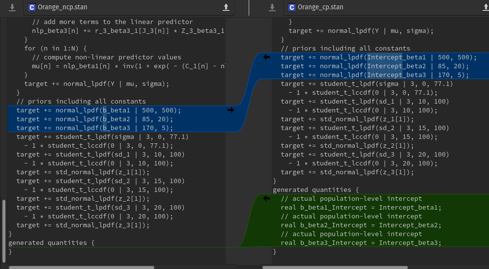
When comparing the STAN code (which is not my strong suit. I’m learning though…), the differences appear to be minimal, and seemingly inconsequential. I can see how they would differ when there would be several covariates, but in this case, as there is only an intercept, the b values are simply set to the intercept at the end.

So, as I understand, for a CP, we should have theta ~ normal(mu, tau), while for an NCP, we should have theta ~ mu + tau * eta , where eta ~ normal(0 , 1). So, in brms, as far as I understand, eta is represented by z_*, and tau is represented by sd_*. Please do correct me if I’m wrong. But in a CP, I would not have expected to see the z_* values represented here? This seems to be a centred parameterisation of the mean, but not of the SD. Is that correct? And is there a way of doing the full CP?

Here are some of the diffs between the STAN code:

Lastly, if I would like to examine the funnel geometry in eta (or in z_*) in brms, I can’t figure out how to look at it. It doesn’t seem to be in the posterior?

Thanks so much in advance for any help or advice!

brms_parameterisation[rmd2r].R (2.7 KB)
Orange_cp.stan (3.9 KB) Orange_ncp.stan (3.9 KB)

3 Likes

Little update about my extra question at the end above, regarding how to look at the posterior of z_*. I still can’t figure out how to get posterior samples for z_* for the default brm() call, but if I use backend = "cmdstanr", then suddenly all the z_* parameters appear in my posterior. Not quite sure why the discrepancy, but it solves that problem for me at least!

rstan

rstanfit <- brm(bform, data = dat1, prior = c(prior1, prior2, prior3, 
                                          prior4, prior5, prior6),
            cores=4, backend="rstan")

dimnames(as.array(rstanfit))
$iterations
NULL

$chains
[1] "chain:1" "chain:2" "chain:3" "chain:4"

$parameters
 [1] "b_beta1_Intercept"           "b_beta2_Intercept"           "b_beta3_Intercept"           "sd_group__beta1_Intercept"   "sd_group__beta2_Intercept"   "sd_group__beta3_Intercept"  
 [7] "sigma"                       "r_group__beta1[3,Intercept]" "r_group__beta1[1,Intercept]" "r_group__beta1[5,Intercept]" "r_group__beta1[2,Intercept]" "r_group__beta1[4,Intercept]"
[13] "r_group__beta2[3,Intercept]" "r_group__beta2[1,Intercept]" "r_group__beta2[5,Intercept]" "r_group__beta2[2,Intercept]" "r_group__beta2[4,Intercept]" "r_group__beta3[3,Intercept]"
[19] "r_group__beta3[1,Intercept]" "r_group__beta3[5,Intercept]" "r_group__beta3[2,Intercept]" "r_group__beta3[4,Intercept]" "lp__"  

cmdstanr

cmdstanrfit <- brm(bform, data = dat1, prior = c(prior1, prior2, prior3, 
                                          prior4, prior5, prior6),
            cores=4, backend="cmdstanr")

dimnames(as.array(cmdstanrfit))
$iterations
NULL

$chains
[1] "chain:1" "chain:2" "chain:3" "chain:4"

$parameters
 [1] "b_beta1_Intercept"           "b_beta2_Intercept"           "b_beta3_Intercept"           "sd_group__beta1_Intercept"   "sd_group__beta2_Intercept"   "sd_group__beta3_Intercept"  
 [7] "sigma"                       "r_group__beta1[3,Intercept]" "r_group__beta1[1,Intercept]" "r_group__beta1[5,Intercept]" "r_group__beta1[2,Intercept]" "r_group__beta1[4,Intercept]"
[13] "r_group__beta2[3,Intercept]" "r_group__beta2[1,Intercept]" "r_group__beta2[5,Intercept]" "r_group__beta2[2,Intercept]" "r_group__beta2[4,Intercept]" "r_group__beta3[3,Intercept]"
[19] "r_group__beta3[1,Intercept]" "r_group__beta3[5,Intercept]" "r_group__beta3[2,Intercept]" "r_group__beta3[4,Intercept]" "lp__"                        "z_1[1,1]"                   
[25] "z_1[1,2]"                    "z_1[1,3]"                    "z_1[1,4]"                    "z_1[1,5]"                    "z_2[1,1]"                    "z_2[1,2]"                   
[31] "z_2[1,3]"                    "z_2[1,4]"                    "z_2[1,5]"                    "z_3[1,1]"                    "z_3[1,2]"                    "z_3[1,3]"                   
[37] "z_3[1,4]"                    "z_3[1,5]"                   

brms usually does not store these quantities, but I do not exclude them yet in cmdstanr for technical reasons. This will change in the future though.

Hi Paul,

Thanks so much for the response! Sorry to be a bit slow to get back to you - I’ve been away this week.

To follow up:

  1. I understand that the z_* parameters are not directly utilised for interpretation of the model, but, from my understanding, this is an important place to check for pathological posterior geometry when making use of the non-centred parameterisation in hierarchical models. From the case study I mentioned earlier, the z_* parameters represent eta[*], which is shown here and here. Or should we be including z_* parameters in our posterior with additions to the generated parameters code block if we really want to look into them?

  2. Is there a way to apply a centred parameterisation with brms in which not only the location, but the scale is also centred (i.e. no z_* parameters ), either using lf() or stanvar(), or some other way? Or ought I to start look into modifying the generated STAN code and running it with cmdstanr directly? Of course brms makes everything so much easier and so much more convenient, so I’d love to stay with it if at all possible, but I also understand that supporting any kind of model configuration or parameterisation is highly burdensome for you as the maintainer of the package. Or is something planned or in the works? If so, I could probably help to contribute if there were to be something planned (especially allowing centring of some random effects and not of others).

Thanks so much for the help!

2 Likes