Taking the maximum of a vector (with uncertainty), or (equally) detecting locations of deviation from a normal distribution

Hi Stan folks,

I have a model where I’m trying to do a regression on the maximum value of a set of vectors. That is, there are 36 birds, each with a set of song pitches, and I want to look at the maximum song pitch for each bird, with a regression against its behavior/physiology/etc,. Naturally, the more measurements in a vector, the better we know what the true maximum value is. I would love to hear your thoughts about how to get a “Bayesian maximum” value out of these that includes uncertainty (with less uncertainty the more measurements we have). I’ve thought about fitting a normal and taking the mean minus two SD, but this feels very hacky, and isn’t actually doing what I want it to do at all. A qqnorm plot shows that a normal distribution is the right choice for the data (created by rescaling all of the birds’ song pitches to within-bird z-scores, and then plotting those together—hopefully that was an appropriate choice).

If they follow a normal distribution, there isn’t really a “true maximum”, because the normal distribution has infinite support. But in reality, we know that birds have maximum pitches that they physically cannot sing above (hopefully limited by their behavior/physiology/etc., since that’s what I’m testing), and perhaps that’s what we’re seeing with the negative deviation from normal in the top right of the qqnorm plot. Looking at it like this, the deviation from normal is probably the signal that I’m trying to get at, because is shows that behavior/physiology/etc. limits maximum frequency, which is the question I want to ask. What is the best way of getting the location of the deviation-from-normal, which I would then use as a response variable?

I was originally planning on making a custom distribution of a normal distribution masked by a logistic, where the logistic’s position relative to the normal distribution is what we’re doing the regression on. That is, there’s a fixed normal distribution with one mu and one sigma, and then there’s a moving logistic masking the distribution, and the position of the logistic is a linear regression of the predictor variables, like this:

target += normal_lpdf(pitch | mu, sigma) + log(logistic(predictor_variables))

Does this make sense? Is this likely to be an identifiable model?

In case it’s relevant, here’s a table of the number of birds with each number of measurements (e.g. 3 birds have only one song measurement each. 4 have 2 measurements. 9 birds have 10 or more measurements each):

   `Number of measurements` `Number of birds`
                      <int>             <int>
 1                        1                 3
 2                        2                 4
 3                        3                 3
 4                        4                 6
 5                        5                 2
 6                        6                 3
 7                        7                 1
 8                        8                 2
 9                        9                 2
10                       10                 1
11                       11                 3
12                       13                 1
13                       15                 2
14                       18                 1
15                       19                 1
16                       20                 1

Thank you all in advance!

I believe I have solved this problem by creating the model I described above. That model has unrelated fitting issues, so I’ll address those in a new post.

I suggest using order statistics. You can directly model the PDF of the maximum of n realizations from an iid density as f_{(n)}(x) = n f(x) F(x)^{n-1}.

@spinkney can you provide a sketch of how to use this approach to achieve the OP’s inference goals? From what I understand, the OP has access to all of the data, not just the maxima, but wants to estimate a model that predicts the likely position of the maximum (ideally not the maximum value in the sample, but rather the actual underlying physiological maximum for the bird that produce the sample).

@maxgotts it doesn’t surprise me that the model you’ve selected has problems sampling, mainly because flexible inference on the shapes of the tails of distributions is very hard (it requires a LOT of data, since most of the data say nothing about the shape of the tail). If you have a 2-parameter logistic, for example, then those are 2 parameters that are ONLY informed by the tail. And in this setting, you need to be especially careful, because you might well find that data in the tail are so sparse that the model would “rather” use the logistic to make some minor touch-ups to deal with slight asymmetries in the bulk of the distribution. This is another pitfall of using parametric inference to learn about the extreme tails of a distribution: unless you’re sure that you have the response distribution is perfectly specified, then the parameters that provide the best fit to the bulk of the distribution (where all the data are) may not be the parameters that provide accurate inference on what’s happening out in the tail.

Given your challenge of estimating the properties of extreme tails of distributions, you really only have two choices. One is to fit a parametric response distribution wherein the tail behavior is governed by parameters that are themselves strongly informed by the bulk of the distribution. This can provide confident inference in the absence of having lots of data, but only if the parametric assumptions are strongly justified, including out in the tail. It sounds to me like you’re not really in this regime. The other is to try to fit something flexible to the tail. Your logistic-masked-normal is an example of a distribution where potentially 2 parameters are (ideally) informed only by data way out in the tail. Obviously this requires a lot of data. You could also take nonparameteric quantile-based approaches (like how we estimate percentiles such as 90, 95, 99, 99.9 from samples when summarizing MCMC posteriors). Again, this requires a LOT of data. One nice thing about this approach is that it makes very explicit the trade-off between how much data you have and how far out into the tail you feel you need to push your inference. For example, 10 samples is already enough to have a pretty clear idea of the median, but doesn’t even begin to constrain likely values of the 99th percentile (except by providing a lower bound for likely values).

We can treat the sample max as the lower bound distribution of the maximum since the maximum must be at least as big as the largest value in each sample. In parameters declare the truncation points with this lower bound, something like in Truncated or Censored Data.

I’d probably model this hierarchically given that qqplot. Assume some hyper population for all replications then for each bird estimate the bird specific distribution. We can see if the variance is constant across bird distributions or gets smaller for larger differences from the hyper mean - birds with high average pitch relative to the pop. are further constrained to have even higher pitch as the max for physical reasons.

Thank you both @spinkney and @jsocolar for this conversation, I really appreciate both of your recommendations.

1. Current Model (not for help debugging, but for inspiration)
I thought I’d mention the model I’m using right now, since it’s somewhat working:

real masked_l_pdf(vector x, real mu, real sigma, vector nu, real lambda, real sign) {
        // https://www.desmos.com/calculator/dmdknl0tnw
        // x: is the value pulled from the distribution
        // mu: is the location of the normal distribution
        // sigma: is the SD of the normal distribution
        // nu: is the vector of locations of the sigmoid masks
        // lambda: is the steepness of the sigmoid mask (be careful -- sigma and lambda are weakly identifiable)
        // sign: is the constant that chooses which side is open (-1 = left open, +1 = right open)

        vector[size(x)] log_sigmoid =  -log1p_exp(-sign*(x-nu)*lambda);
        vector[size(x)] log_normal = -log(sigma)-0.5*square((x-mu)/sigma);
        
        return sum(log_sigmoid + log_normal);
    }

This is the log PDF of my sigmoid-masked normal distribution. As you said @jsocolar, it has two parameters that it needs to fit, and very little data with which to do so. At the moment, I’m just setting lambda=10 (high steepness), so it’s only trying to fit nu, the position parameter. Here’s how I do that:

model {
  mu ~ normal(0,1); // Weakly informative prior
  sigma ~ normal(1,1); // Weakly informative prior
  beta ~ normal(0,3); // Uninformative prior

  vector[nBird] nu = beta*behavior; // Regression occurs here

  target += masked_l_pdf(
    pitch,
    mu,
    sigma,
    nu[pitch_bird],
    lambda/sigma, // Divide by sigma so that steepness is sigma-invariant
    -1.0 // Left-open sigmoid
  );
}

The issue with this model—and I’m not sure how much of an issue this is—is that it takes all of the data without any form of multilevel structuring. This means that I have ~260 individual pitch measurements (unevenly distributed over 36 birds) to fit the “tail” of this distribution. I put “tail” in quotes because there isn’t just 1 tail, it’s actually a moving tail based on the value of the behavior. In this model, beta is underestimated (but its sign is correctly retrodicted), but mu and sigma are properly retrodicted.

To make this multilevel, I tried this instead:

parameters {
  real mu;
  real<lower=0> sigma;
  vector[nBird] nu;
  real beta;
  real<lower=0> error;
}
model {
  // Fit the masked normal for each bird
  mu ~ normal(0,1); // Weakly informative prior
  sigma ~ normal(1,1); // Weakly informative prior

  target += masked_l_pdf(
    pitch,
    mu,
    sigma,
    nu[pitch_bird],
    lambda/sigma, // To put steepness in standard units
    -1.0
  );
  
  // Fit the regression on behavior by nu
  beta ~ normal(0,3); // Uninformative prior
  error ~ normal(1,1); // Weakly informative prior
  nu ~ normal(beta*behavior, error); // Do the regression
}

Here, nu is fit for each bird, and then I directly do the regression on nu by behavior. This makes more sense, but suddenly I have much less data (at most 20 points, but often closer to 5-10) to fit the tail for each bird (yikes!). Add to this the underestimation in beta from my first model, and this model completely fails to retrodict beta.

Questions: How much of an issue is my first model, without a multilevel structure? I go back on forth on this. Clearly it isn’t great, but is it as indefensible as e.g. doing a straight linear regression on pitch by behavior value? Is there an argument to be made about using the data we have as effectively as possible (i.e. we can always make a model more mechanistic and “accurate” than the last one but there is not enough data in the world to fit effectively, therefore at some point we have to make a trade-off between a “good” model and one that actually informs us about the world)? If I were to use this non-multilevel model, how bad would that actually be? I’m open to hearing “no, don’t do this”—I want to do good, defensible statistics to understand the world better. But I’d also like to build a model that my data can actually fit.

2. Two Truncated Normal Models
I liked the idea of an unknown truncation approach recommended by @spinkney. I would be very curious to see if a high-steepness (i.e. lambda=50 as a constant not a parameter) sigmoid-masked normal would be a better fit than a truncated normal, since that fits better with the physiological mechanism (the birds are attempting to sing higher, but are physiologically limited by a logistic-type mask)—or maybe these would be functionally identical, I’m not sure.

This high-steepness model would be the multilevel model from above, just with a lambda much higher than I was anticipating using. It fails to retrodict beta, but happily retrodicts mu and sigma.

Here’s my implementation of the multilevel truncated normal model @spinkney described. I’m not quite sure I understood everything you said, so I’ve kept it relatively simple at the moment with a bird-level truncation and a regression on truncation-point and behavior, and a constant mu and sigma shared between all birds.

parameters {
  real mu;
  real<lower=0> sigma;
  vector<lower=max_pitch>[nBird] upsilon; // max_pitch is an nBird-length vector from data
  real beta;
  real<lower=0> error;
}
model {
  // Fit the truncated normal for each bird
  mu ~ normal(0,1); // Weakly informative prior
  sigma ~ normal(1,1); // Weakly informative prior

  for (i in 1:nPitch) { // I'm not sure if I can just do pitch ~ normal(mu, sigma) T[,upsilon[pitch_bird]]?
    pitch[i] ~ normal(mu, sigma) T[,upsilon[pitch_bird[i]]];
  }
  
  // Fit the regression on behavior by upsilon
  beta ~ normal(0,2); // Weakly informative prior (not sure how to do this properly)
  error ~ normal(1,1); // Weakly informative prior
  upsilon ~ normal(beta*behavior, error); // Do the regression
}

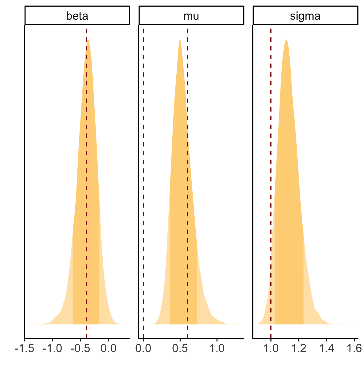
This does a much better job of retrodicting beta, but struggles with mu and sigma:


This is using the same data I used for the previous models (i.e., generated from a sigmoid-masked normal with mu=0, sigma=1, lambda=10, and nu for each bird being a linear relationship of beta_behavior=-0.4, and beta0=0.6. The red lines are beta_behavior for beta, beta0-mu and mu for mu (I wasn’t sure what was the right choice for mu here), and sigma for sigma.

Questions: @spinkney does this look like the model you were picturing in your comment?

3. Quantile Approach
Based on my understanding of @jsocolar’s comment, I don’t think I have enough data to even attempt a quantile-based approach. For some birds I have but a single data point (unfortunately, it was really, really hard to get good recordings of these birds in the field), so I’m not sure any quantile (except median) would be a real value for every bird. Am I understanding your comment correctly?

Thank you again both for your thoughts on this slightly strange model I’m trying to build. I really, really appreciate all of your help with this!!

It might be worth taking a step back and thinking about the biological system here. I could imagine you could be working with highly stereotyped homologous vocalizations (think of loudsongs from an Antpitta or flight calls from a Parulid). At the other end of the spectrum, I could imagine you’re working with extremely variable and/or non-homologous vocalizations (think of short song fragments from a Lyrebird, or a haphazard mix of songs and various calls).

A crucial thing to notice is that in the latter regime, a single sample tells you nothing (other than a lower bound) about the likely value of the maximum. I’m hoping you’re not in this regime, but I think it’s worth harping on a bit more. How many 2-second Lawrence’s Thrush fragments would you need in order to begin to feel confident about a max frequency? How many recordings of a Northern Saw-whet Owl would you need to sift through (listening to loudsong after loudsong) before you’d be likely to stumble on the chitter call with a peak frequency ~3x higher?

What I’m driving at here is that with low sample sizes, this whole exercise only really works if the within-subject variances are low enough that a small sample size of recordings tells you something about the subject-specific maximum. I don’t want to be discouraging, and indeed I’m hoping that you are in the low-variance regime, where you might find yourself when analyzing homologous, stereotyped vocalizations (or if vocalizations aren’t stereotyped, maybe you can get something similar if “one sample” is actually an extended cut, and the sounds are still homologous). In this low-variance regime, I do just want to float the possibility that it might not actually be necessary to estimate subject-specific maxima. Why not just take the average over samples (within a subject) of the peak per-sample frequency? That’s the sort of vocal trait that is routinely quantitatively scored in bioacoustic analyses of birdsong, and it’s likely to be waaay less of a headache than all of this fiddly tinkering with small-sample inference on the tails of distributions – fiddly tinkering that I’m afraid might come to naught anyway, since there’s really no such thing as small-sample inference on distributional tails except via techniques that are absurdly sensitive to misspecification of the response distribution.

2 Likes

Hi @jsocolar! I really appreciate your comments, and it brings up some thoughts I’ve been considering too.

TL;DR: I took your advice, and it totally worked. Good ole +(1|warbler) to the rescue!

I completely agree with you—the system is incredibly relevant for this question (and whether it’s well-posed at all). I am working with is warbler song. For this particular species, they have 2 kinds of song, one of which is known to have higher maximum frequencies (‘Type I’ songs, which are the ones I’m interested in, but it’s incredibly hard to distinguish the two without immense field effort, unfortunately). I have heard from biologists (who study birdsong) at my university that parulid Type I songs are probably at warblers’ physiological limits, but I haven’t actually read that myself.

In my dataset, the peak frequencies of these songs (i.e. the frequency of the periodogram with the highest value) are a high-variance regime, where individuals’ songs variances are on par with population-wide variances (which makes me believe that the warblers are all trying to go for the same song frequencies overall, more or less). The high frequency (i.e. maximum frequency of an individual song) appears to be in a low(er)-variance regime, as you can see below:

I’ve just run the pitch ~ behavior + (1|warbler) type model, as you described, and it completely worked. I was hoping to make a more mechanistic model, but that might not actually be possible with the data I have, and looking again at the figure above, I think you’re right that it should actually provide the same results. As a sanity check, we expect PC1 to have a negative impact on pitch (if any), PC2 to have any impact, and PC3 to have a negative impact (if any). So this fits with what I was imagining I might see!

Thank you so much @jsocolar—I feel silly I didn’t try this straight away, and I’m really grateful for talking to you about this! How would you like to be included in my acknowledgements (and same question for @spinkney)?

1 Like

@jsocolar nice work! The low variance scenario with strong assumptions is really the only way this will work to estimate those tails with any confidence in low samples.

In regards to the truncation model I think if you set mu to 0 and with some clever tinkering of the variances it will recover the parameters. Again though you’ll be making some assumptions about the process.

Acknowledgements are always nice! If you message me I’ll send you my contact details.

1 Like