I am trying to estimate a repeated measures model with individual-level random intercepts and correlated random slopes partitioned into genetic effects G and environmental effects E. The genetic effects are scaled with fixed row-wise relatedness matrix A, which is relatively sparse. The environmental effects are i.i.d. and meant to simply soak up any unobserved individual heterogeneity not captured by the fixed covariance genetic effects. The response model is specified by the sum G + E, which is making it difficult for identification of the distinct standard deviations and correlations of the G and E effects. The model does a somewhat good job of returning simulated SDs despite sampling quite poorly (with low bulk and tail ESS), but the correlations seem to jump around haphazardly.
I’ve experimented with implementing basic prior regularization and some constraints on the parameters, but I’m hoping I’ve missed more effective strategies for enhancing identification. My code is below. Note that I take advantage of a matrix normal parameterization of the genetic effects to avoid direct computation of the Kronecker product G %x% A.
data {
  int<lower=1> N; //number of observations
  int<lower=0> I; //number of individuals
  int<lower=0> M; //number of genetic effects
  int<lower=0> E; //number of environment effects
  int<lower=1> id_j[N]; //index of individual observations
  matrix[I,I] Amat; //genetic relatedness matrix
  vector[N] X1; //covariate
  real Y[N]; //normal response
}

transformed data{
   matrix[I,I] LA = cholesky_decompose(Amat); //lower-triangle A matrix
   real conditional_mean0 = 0; //fixed global intercept
}

parameters {
  real<lower=-1,upper=1> conditional_mean1; //expectation for subject slopes
  vector<lower=0>[M] sdG_U; //genetic effect SDs
  vector<lower=0>[E] sdE_U; //environment effect SDs
  real<lower=0> sd_R; //residual SD
  cholesky_factor_corr[M] LG_u; //genetic effect correlations
  cholesky_factor_corr[E] LE_u; //environment effect correlations
  matrix[I,M] std_devG; //genetic deviations
  matrix[I,E] std_devE; //environment deviations
}

transformed parameters {
  matrix[I, M] G_re; //genetic random effects (G_intercept, G_slope)
  matrix[I, E] E_re; //environment random effects (E_intercept, E_slope)
  vector[I] P0; //phenotypic random intercepts (G + E)
  vector[I] P1; //phenotypic random slopes (G + E)

 //matrix normal sampling of genetic effects
  G_re = LA * std_devG  * diag_pre_multiply(sdG_U, LG_u) ;
 //environment effects
  E_re = std_devE * diag_pre_multiply(sdE_U, LE_u) ;
//phenotypic effects (centered on global intercept and slope)
  P0 = rep_vector(conditional_mean0, I) + col(G_re,1) + col(E_re,1);
  P1 = rep_vector(conditional_mean1, I) + col(G_re,2) + col(E_re,2);
}

model{
  conditional_mean1 ~ std_normal();
  to_vector(std_devG)~std_normal();
  to_vector(std_devE)~std_normal();
  LG_u ~ lkj_corr_cholesky(3);
  LE_u ~ lkj_corr_cholesky(3);
  to_vector(sdG_U) ~ exponential(3);
  to_vector(sdE_U) ~ exponential(3);
  sd_R ~ exponential(3); //residual sd

//response Y ~ G_int + E_int + (G_slope + E_slope)*X1
  Y ~ normal( P0[id_j] + P1[id_j].*X1, sd_R);
}
Here are posterior plots indicative of the identification issues for the G and E SDs and correlations.
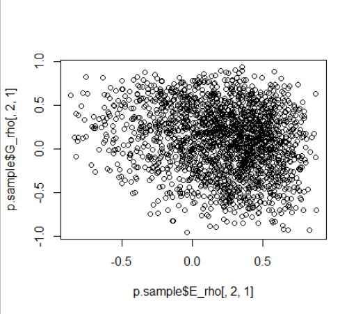
I simulated G and E correlations of large magnitude and opposite sign (-0.5 and 0.5 respectively).
Thanks for your help!
1 Like
Hi,
sorry for taking quite long to respond.
One thing I’ve found useful in a different context where I also had two sources of variability that were hard to distinguish was to have a parameter for total variability and then a proportion of the variability to be accounted for by one of the components, e.g. (for just one sd parameter):
parameters {
  real<lower=0> total_sd;
  real<lower=0,upper=1> varianceG_frac;
}

transformed parameters {
  //simplified from sqrt((total_sd^ 2) * varianceG_frac)
  real<lower=0> sdG = total_sd * sqrt(varianceG_frac);
  //simplified sqrt((total_sd^ 2) * (1 - varianceG_frac))
  real<lower=0> sdE = total_sd * sqrt(1 - varianceG_frac);
}
Note that we need to transform from sd to variance, as variance is a linear operator while sd is not.
This way total_sd becomes usually well identified and independent of varianceG_frac (in the model I’ve used the posterior for this parameter was basically uniform over [0,1] indicating that we couldn’t learn the decomposition, so the model is effectively integrating it out - and the sampling worked quite well).
Does that make sense? And do you think this answers you inquiry?
Not sure if you could decompose the whole covariance matrix this way, but it might be possible… (my linear algebra is too rusty for that). Or maybe just doing this for the standard deviations would be enough.
Best of luck with your model!
2 Likes
Thanks Martin, this is a great idea that had not occurred to me. It seems quite sensible in this context. I will give it a shot and report back!
A brief note as well for anyone who visits this topic in the mean time. The code above is missing transpose operations on the matrix normal parameterization of the random effects.
 //matrix normal sampling of genetic effects
  G_re = LA * std_devG  * diag_pre_multiply(sdG_U, LG_u) ;
 //environment effects
  E_re = std_devE * diag_pre_multiply(sdE_U, LE_u) ;
Should be
 //matrix normal sampling of genetic effects
  G_re = LA * std_devG  * diag_pre_multiply(sdG_U, LG_u)' ;
 //environment effects
  E_re = std_devE * diag_pre_multiply(sdE_U, LE_u)';
I’ll post updated code once I’ve attempted Martin’s suggestion.
1 Like
Thank you again Martin for this suggestion. I’ve now implemented the parameterization you suggested and found the model to be doing much better. The model is sampling faster and the identifiability of the random effects has been improved overall. A conceptual upshot of your approach is that, in this simple case, the varianceG_frac parameter can be interpreted as the heritability coefficient (h^2).
Here is my updated code. I’m not confident about the best prior for the varianceG_frac parameter (labelled h2 below), but I have opted for regularization toward 0 with a Beta(1,5) prior.
data {
  int<lower=1> N; //number of observations
  int<lower=0> I; //number of individuals
  int<lower=0> M; //number of latent phenotypic traits
  int<lower=1> id_j[N]; //index of individual observations
  matrix[I,I] Amat; //genetic relatedness matrix
  vector[N] X1; //partner phenotype covariate
  real Y[N]; //normal response
}

transformed data{
   matrix[I,I] LA = cholesky_decompose(Amat); //lower-triangle A matrix
}

parameters {
  real conditional_mean0; //expectation for subject intercepts
  real conditional_mean1; //expectation for subject slopes
  real<lower=0> sd_R; //residual SD
  cholesky_factor_corr[M] LG; //genetic effect correlations
  cholesky_factor_corr[M] LE; //environment effect correlations
  vector<lower=0>[M] total_sd; //total phenotypic SD
  vector<lower=0,upper=1>[M] h2; //heritability

  matrix[I,M] std_devG; //genetic deviations
  matrix[I,M] std_devE; //environment deviations
}

transformed parameters {
  vector<lower=0>[M] sdG; //standard deviation of G effects
  vector<lower=0>[M] sdE; //standard deviation of E effects
  matrix[I, M] G_re; //subject genetic random effects
  matrix[I, M] E_re; //subject environment random effects
  vector[I] P0; //subject phenotype random intercepts (G + E)
  vector[I] P1; //subject phenotype random slopes (G + E)

  //standard deviations of genetic effects (total SD * proportion G SD)
  //simplified from sqrt ( total variance * h2 )
  sdG[1] = total_sd[1] * sqrt(h2[1]);
  sdG[2] = total_sd[2] * sqrt(h2[2]);

  //standard deviations of environmental effects (total SD * proportion E SD)
  sdE[1] = total_sd[1] * sqrt(1 - h2[1]);
  sdE[2] = total_sd[2] * sqrt(1 - h2[2]);

  //matrix normal sampling of genetic effects
  G_re =  LA * std_devG  * diag_pre_multiply(sdG, LG)' ;

  //environment effects
  E_re = std_devE * diag_pre_multiply(sdE, LE)' ;

  //phenotypic effects (centered on global intercept and slope)
  P0 = rep_vector(conditional_mean0, I) + col(G_re,1) + col(E_re,1);
  P1 = rep_vector(conditional_mean1, I) + col(G_re,2) + col(E_re,2);
}

model{
  conditional_mean0 ~ std_normal();
  conditional_mean1 ~ std_normal();
  to_vector(std_devG)~std_normal();
  to_vector(std_devE)~std_normal();
  LG ~ lkj_corr_cholesky(3);
  LE ~ lkj_corr_cholesky(3);
  to_vector(total_sd) ~ std_normal();
  h2 ~  beta(1,5);
  sd_R ~ exponential(3);

  Y ~ normal( P0[id_j] + P1[id_j].*X1, sd_R);
}
I will be using this approach in a forthcoming publication, so I will link to the work here when it is available for future readers of the thread.
I sincerely appreciate your help!
1 Like
