Abnormally low variance for one random-effect in a cross-classified hierarchical linear model (with correlated random effects)

[jflournoy]

I’ve written a hierarchical general linear model with two simultaneous equations that are models of two vectors of observed data that come from the same participants. There are several parameters which are allowed to vary across participants, and these are modeled as arising from a multivariate normal distribution implemented through the non-centered parameterization. In addition to the participant-level grouping factor, there is another crossed grouping factor called roi (every participant has data from every level of this other grouping factor, and every level of that grouping factor has data from every participant). The same parameters are allowed to vary across the roi factor and are similarly modeled.

Here’s a snippet of the stan code (it’s a pretty straightforward modification of Matti’s code in the bmlm package (https://github.com/mvuorre/bmlm):

parameters{
    vector[P] gammas;                    //Population level effects
    // Regression Y on X and M
    //     1 real dy;                    // Intercept
    //     2 real cp;                    // X to Y effect
    //     3 real b;                     // M to Y effect
    //     4 real ty;                    // t to Y effect
    // Regression M on X
    //     5 real dm;                    // Intercept
    //     6 real a;                     // X to M effect
    //     7 real tm;                    // t to M effect

    // Correlation matrix and SDs of participant-level varying effects
    cholesky_factor_corr[P] L_Omega_id;
    vector<lower=0>[P] Tau_id;
    // Correlation matrix and SDs of roi-level varying effects
    cholesky_factor_corr[P] L_Omega_roi;
    vector<lower=0>[P] Tau_roi;

    // Standardized varying effects
    matrix[P, J] z_U;
    matrix[P, K] z_V;           //shardable over K ROIS
    vector[Ly] ybeta;           // ID-varying covariates to Y
    vector[Lm] mbeta;           // ID-varying covariates to M
    real<lower=0> sigma_m;      // Residual
    real<lower=0> sigma_y;      // Residual
}
transformed parameters {
    // Participant-level varying effects
    matrix[J, P] U;
    // ROI-level varying effects
    matrix[K, P] V;
    U = (diag_pre_multiply(Tau_id, L_Omega_id) * z_U)';
    V = (diag_pre_multiply(Tau_roi, L_Omega_roi) * z_V)';
}
model {
    // Means of linear models
    vector[N] mu_y;
    vector[N] mu_m;
    // Regression parameter priors
    gammas ~ normal(0, prior_bs);
    ybeta ~ normal(0, prior_ybeta);
    mbeta ~ normal(0, prior_mbeta);
    // SDs and correlation matrix ID-varying
    Tau_id ~ cauchy(0, prior_id_taus); 
    L_Omega_id ~ lkj_corr_cholesky(prior_id_lkj_shape);
    // SDs and correlation matrix ROI-varying
    Tau_roi ~ cauchy(0, prior_roi_taus); 
    L_Omega_roi ~ lkj_corr_cholesky(prior_roi_lkj_shape);

    // Allow vectorized sampling of varying effects via stdzd z_U, z_V
    to_vector(z_U) ~ normal(0, 1);
    to_vector(z_V) ~ normal(0, 1);

    mu_y = (gammas[2] + U[id, 2] + V[roi, 2]) .* X +       // cp
           (gammas[3] + U[id, 3] + V[roi, 3]) .* M +       // b
           (gammas[4] + U[id, 4] + V[roi, 4]) .* Time +    // ty
           (gammas[1] + Cy*ybeta + U[id, 1] + V[roi, 1]);  // dy
    mu_m = (gammas[6] + U[id, 6] + V[roi, 6]) .* X +       // a
           (gammas[7] + U[id, 7] + V[roi, 7]) .* Time +    // tm
           (gammas[5] + Cm*mbeta + U[id, 5] + V[roi, 5]);  // dm
    // Data model
    Y ~ normal(mu_y, sigma_y);
    M ~ normal(mu_m, sigma_m);
}

The problem

The problem I’m facing is that, when I simulate data with with known parameters and fit this model, a subset of the random effects in the V matrix are estimated with extremely squashed variance. Here’s a plot of the data-generating random effects and the poster means (the black line is identity). It’s consistently the random “b” parameter (corresponding to V[roi, 3], actually computed for these plots as gammas[3] + V[roi, 3]). Correspondingly, Tau_roi[3] is much smaller 0.0085 versus 1.00.

The same thing is actually happening with the same parameter with regard to the id grouping factor (the U matrix). That is, the mean posterior Tau_id[3] is way smaller than the data-generating Tau_id[3], but it’s not having quite as detrimental effect on the rank-order of U[,3].

I’ve done a bunch of proof-reading of my model and I can’t find anything that is wrong at the level of a typo. I’m hoping that this kind of problem is something that is fairly recognizable from the information I’ve provided. I should say that the diagnose command says all is okay as far as tree-depth, divergent transitions, effective samples, and split rhat.

[martinmodrak]

Sorry, can’t look into this now, but maybe @mike-lawrence is not busy and can help?

[mike-lawrence]

Just to summarize:

So you have two outcome variables, Y & M, and, in addition to modelling the effect of a few predictors on both, you’re also modelling the influence of M on Y. You have two variables, id and roi that cause variability in the influence of M on Y that you’re modelling hierarchically, and when you simulate data with moderate variability induced by these variables (x-axis of your plots), the posterior for these seem to have much lower variability than expected (y-axis of your plots). And the posterior distribution for the variability parameters, Tau_id[3] and 'Tau_roi[3]` concentrate on very low values.

Presumably you’re not getting any model diagnostic warnings?

Note that you currently don’t have any prior on the residual parameters sigma_y and sigma_m (or, you have implicit uniform(0,infinity) prior); you might want to use a more informed prior. For residuals, it’s common to use normal(0,sd) with an informed sd, but I don’t find such peaked-at-zero priors credible as they imply peak credence for zero measurement noise. I like the weibull as a zero-at-zero prior, but I’ve also seen gammas; I just find it easier to think about the parameters in the weibull.

You’re also using half-cauchy priors on the across-id and across-roi variance parameters. For these I think peaked-at-zero are more defensible, but folks have lately been arguing against heavy-tail priors like cauchy.

I don’t think any of those tweaks will address your observation of non-calibration (I think that’s the term when you evaluate whether the model can recover simulated data) though. I’m having trouble coming up with any ideas on that score, so we might need to call in heavier hitters than me for that. Maybe confirm that there are no diagnostic warnings, and if not we’ll tag someone else in?

[jflournoy]

@mike-lawrence

Just to summarize:

Your summary is exactly right. Thank you.

@mike-lawrence

Presumably you’re not getting any model diagnostic warnings?

That’s correct, I don’t have any diagnostic warnings.

@mike-lawrence

Note that you currently don’t have any prior on the residual parameters sigma_y and sigma_m…

I’ve updated the model to include better priors on these parameters – exponential(1), which I think satisfies the zero-at-zero criterion. I did not change the half-cauchy. I did slightly repramaterize according to the suggestion in the manual, e.g.:

vector<lower=0,upper=pi()/2>[P] Tau_id_unif;
...
for (p in 1:P) {
      Tau_id[p] = prior_id_taus * tan(Tau_id_unif[p]);
}

@mike-lawrence

I’m having trouble coming up with any ideas on that score, so we might need to call in heavier hitters than me for that.

I set up and am running a more reproducible example. Currently waiting on fitting a chain to each of 10 simulated data sets. I’ll report back on the outcome and link to the repository when those are done.

[mike-lawrence]

@jflournoy

I’ve updated the model to include better priors on these parameters – exponential(1) , which I think satisfies the zero-at-zero criterion.

Unless I’m mistaken, doesn’t an exponential distribution increase in density as you approach zero?

[jflournoy]

@mike-lawrence

doesn’t an exponential distribution increase in density as you approach zero

Yes, but I think probability at 0 is 0 (e.g., in R, pexp(0) = 0). I will try changing it to weibull with shape = 1.5 (which looks like it pulls the peak away from 0) after this run is done to see if that makes a difference.

[mike-lawrence]

Ah, yes, I guess I should say “zero-near-zero” rather than simply “zero-at-zero”, as technically all truncated distributions are zero-at-zero. The point is to choose a distribution that reflects the prior belief that zero or very small values for measurement error are relatively incredible, slightly larger values are more credible, very large values are relatively less credible again, etc. That’s why I like the weibull, though a shifted normal would work too.

I also failed to specify what shape of weibull, and you correctly surmised that you’d want a shape>1, as weibull(1,1) is the same as exponential(1). Merely because I like whole numbers, I like to use weibull(2,1) when the data has been scaled to have unit variance

[jflournoy]

I’ve created a reporducible example with data and fits. I have not updated with the weibull specification. Additionally, not all chains finished without diagnostic warnings, so I need to rerun this all to update those things. In the meantime, the results are much the same as I’ve gotten before: very constrained random effects (group-varying parameter) variance for a handful of parameters.

Here is the repository: https://github.com/jflournoy/mlmed_example

A brief exploration of the fits from 4 simulations is here: https://jflournoy.github.io/mlmed_example/sim_fit_results.html#all_fits_to_simulated_data (see below for one of the plots if you don’t feel like clicking through).

The full stan code is here for your convenience:

// Y Equation
//   level 1:
//     y ~ normal(dy_ + ty_*TIME + cp_*X + b_*M, sigma_y)
//   level 2:
//     dy_ = dy + Cy*ybeta + U[id, 4] + V[roi, 4]
//     ty_ = ty + U[id, 6] + V[roi, 6]
//     cp_ = cp + U[id, 1] + V[roi, 1]
//     b_ = b + U[id, 2] + V[roi, 2]
//
// M Equation
//   level 1:
//     m ~ normal(dm_ + tm_*TIME + a_*X, sigma_m)
//   level 2:
//     dm_ = dm + Cm*mbeta + U[id, 5] + V[roi, 5]
//     tm_ = tm + U[id, 7] + V[roi, 7]
//     a_ = a + U[id, 3] + V[roi, 3]

data {
    int<lower=1> N;             // Number of observations
    int<lower=1> J;             // Number of participants
    int<lower=1> K;             // Number of ROIs
    int<lower=1> Ly;            // Number of participant-varying covariates, y equation
    int<lower=1> Lm;            // Number of participant-varying covariates, m equation
    int<lower=1,upper=J> id[N]; // Participant IDs
    int<lower=1,upper=K> roi[N];// ROI ids
    vector[N] X;                // Treatment variable
    vector[N] M;                // Mediator
    vector[N] Time;             // Time variable (just de-trending for each J and K)
    matrix[N, Ly] Cy;           // participant/ROI-varying covariates, y equation - we just assume the coefficients for these do not vary by ID or ROI though the values of the variables might differ within participant by ROI, or within ROI by participant
    matrix[N, Lm] Cm;           // participant/ROI-varying covariates, m equation - we just assume the coefficients for these do not vary by ID or ROI though the values of the variables might differ within participant by ROI, or within ROI by participant

    real prior_bs;
    real prior_sigmas;
    //ID Priors
    real prior_id_taus;
    real prior_id_lkj_shape;
    //ROI Priors
    real prior_roi_taus;
    real prior_roi_lkj_shape;
    //ID varying covars Priors
    real prior_ybeta;
    real prior_mbeta;

    int<lower=0,upper=1> SIMULATE; //should we just simulate values?
    vector[N] Y;                // Continuous outcome
}
transformed data{
    int<lower = 0> N_sim = 0;
    int P = 7;                  // Number of person & ROI-varying variables: dm, dy, a,
                                // b, cp, ty, tm. That is, intercept for m and y
                                // equations, a path, b path, c prime path, and 2 time
                                // effects.

    //This keeps us from generating a huge but empty
    //vector if we're not going to put generated
    //quantities in it.
    if(SIMULATE == 1){
      N_sim = N;
    }
}
parameters{
    // Regression Y on X and M
    vector[P] gammas;
    //     1 real dy;           // Intercept
    //     2 real cp;           // X to Y effect
    //     3 real b;            // M to Y effect
    //     4 real ty;           // t to Y effect
    // Regression M on X
    //     5 real dm;           // Intercept
    //     6 real a;            // X to M effect
    //     7 real tm;           // t to M effect
    vector[Ly] ybeta;           // ID-varying covariates to Y
    vector[Lm] mbeta;           // ID-varying covariates to M
    real<lower=0> sigma_m;

    // Correlation matrix and SDs of participant-level varying effects
    cholesky_factor_corr[P] L_Omega_id;
    vector<lower=0,upper=pi()/2>[P] Tau_id_unif;

    // Correlation matrix and SDs of roi-level varying effects
    cholesky_factor_corr[P] L_Omega_roi;
    vector<lower=0,upper=pi()/2>[P] Tau_roi_unif;

    // Standardized varying effects
    matrix[P, J] z_U;
    matrix[P, K] z_V;
    real<lower=0> sigma_y;
}
transformed parameters {
    //Variance scales
    vector<lower=0>[P] Tau_id;
    vector<lower=0>[P] Tau_roi;
    // Participant-level varying effects
    matrix[J, P] U;
    // ROI-level varying effects
    matrix[K, P] V;

    // Tau_id ~ cauchy(0, prior_id_taus);
    // Tau_roi ~ cauchy(0, prior_roi_taus);
    for (p in 1:P) {
      Tau_id[p] = prior_id_taus * tan(Tau_id_unif[p]);
      Tau_roi[p] = prior_roi_taus * tan(Tau_roi_unif[p]);
    }

    U = (diag_pre_multiply(Tau_id, L_Omega_id) * z_U)';
    V = (diag_pre_multiply(Tau_roi, L_Omega_roi) * z_V)';
}
model {
    // Means of linear models
    vector[N] mu_y;
    vector[N] mu_m;
    // Regression parameter priors
    gammas ~ normal(0, prior_bs);
    ybeta ~ normal(0, prior_ybeta);
    mbeta ~ normal(0, prior_mbeta);
    sigma_y ~ exponential(prior_sigmas);
    sigma_m ~ exponential(prior_sigmas);
    L_Omega_id ~ lkj_corr_cholesky(prior_id_lkj_shape);
    L_Omega_roi ~ lkj_corr_cholesky(prior_roi_lkj_shape);

    // Allow vectorized sampling of varying effects via stdzd z_U, z_V
    to_vector(z_U) ~ normal(0, 1);
    to_vector(z_V) ~ normal(0, 1);//shardable over K rois

    if(SIMULATE == 0){
      // Regressions
      //     1 real dy;                    // Intercept
      //     2 real cp;                    // X to Y effect
      //     3 real b;                     // M to Y effect
      //     4 real ty;                    // t to Y effect
      mu_y = (gammas[2]            + U[id, 2] + V[roi, 2]) .* X +
             (gammas[3]            + U[id, 3] + V[roi, 3]) .* M +
             (gammas[4]            + U[id, 4] + V[roi, 4]) .* Time +
             (gammas[1] + Cy*ybeta + U[id, 1] + V[roi, 1]);
      // Regression M on X
      //     5 real dm;                    // Intercept
      //     6 real a;                     // X to M effect
      //     7 real tm;                    // t to M effect
      mu_m = (gammas[6]            + U[id, 6] + V[roi, 6]) .* X +
             (gammas[7]            + U[id, 7] + V[roi, 7]) .* Time +
             (gammas[5] + Cm*mbeta + U[id, 5] + V[roi, 5]);
      // // Data model
      Y ~ normal(mu_y, sigma_y);
      M ~ normal(mu_m, sigma_m);
    }
}
generated quantities{
    //NOTE: Include relevant generated quantities for new ROI-varying effect covariance
    matrix[P, P] Omega_id;         // Correlation matrix
    matrix[P, P] Sigma_id;         // Covariance matrix
    matrix[P, P] Omega_roi;         // Correlation matrix
    matrix[P, P] Sigma_roi;         // Covariance matrix

    // Average mediation parameters
    real covab_id;              // a-b covariance across IDs
    real corrab_id;             // a-b correlation across IDs
    real covab_roi;             // a-b covariance acrosss ROIs
    real corrab_roi;            // a-b correlation acrosss ROIs
    real me;                    // Mediated effect
    real c;                     // Total effect
    real pme;                   // % mediated effect

    // Person-specific mediation parameters
    vector[J] u_a;
    vector[J] u_b;
    vector[J] u_cp;
    vector[J] u_dy;
    vector[J] u_dm;
    vector[J] u_ty;
    vector[J] u_tm;
    vector[J] u_c;
    vector[J] u_me;
    vector[J] u_pme;
    // ROI-specific mediation parameters
    vector[K] v_a;
    vector[K] v_b;
    vector[K] v_cp;
    vector[K] v_dy;
    vector[K] v_dm;
    vector[K] v_ty;
    vector[K] v_tm;
    vector[K] v_c;
    vector[K] v_me;
    vector[K] v_pme;

    // Re-named tau parameters for easy output
    real dy;
    real cp;
    real b;
    real ty;
    real dm;
    real a;
    real tm;

    real tau_id_cp;
    real tau_id_b;
    real tau_id_a;
    real tau_id_dy;
    real tau_id_dm;
    real tau_id_ty;
    real tau_id_tm;
    real tau_roi_cp;
    real tau_roi_b;
    real tau_roi_a;
    real tau_roi_dy;
    real tau_roi_dm;
    real tau_roi_ty;
    real tau_roi_tm;

    real Y_sim[N_sim];
    real M_sim[N_sim];


    // 1 u_intercept_y
    // 2 u_cp (X)
    // 3 u_b  (M)
    // 4 u_ty (Time)
    // 5 u_intercept_m
    // 6 u_a  (X)
    // 7 u_tm (Time)

    tau_id_dy =  Tau_id[1];
    tau_id_cp =  Tau_id[2];
    tau_id_b =   Tau_id[3];
    tau_id_ty =  Tau_id[4];
    tau_id_dm =  Tau_id[5];
    tau_id_a =   Tau_id[6];
    tau_id_tm =  Tau_id[7];
    tau_roi_dy = Tau_roi[1];
    tau_roi_cp = Tau_roi[2];
    tau_roi_b =  Tau_roi[3];
    tau_roi_ty = Tau_roi[4];
    tau_roi_dm = Tau_roi[5];
    tau_roi_a =  Tau_roi[6];
    tau_roi_tm = Tau_roi[7];

    Omega_id = L_Omega_id * L_Omega_id';
    Sigma_id = quad_form_diag(Omega_id, Tau_id);
    Omega_roi = L_Omega_roi * L_Omega_roi';
    Sigma_roi = quad_form_diag(Omega_roi, Tau_roi);

    //NOTE: We need to figure out what is the proper way to
    //      acount for covariance between a and b paths
    //      across both grouping factors (ID and ROI,
    //      crossed, not nested).
    //
    //      I've taken a stab at something that might
    //      be correct but it's a very naive extension
    //      of the case where there is only one grouping
    //      factor.
    covab_id = Sigma_id[6,3];
    corrab_id = Omega_id[6,3];
    covab_roi = Sigma_roi[6,3];
    corrab_roi = Omega_roi[6,3];
    // vector[P] gammas;
    // //     1 real dy;                    // Intercept
    // //     2 real cp;                    // X to Y effect
    // //     3 real b;                     // M to Y effect
    // //     4 real ty;                    // t to Y effect
    // // Regression M on X
    // //     5 real dm;                    // Intercept
    // //     6 real a;                     // X to M effect
    // //     7 real tm;                    // t to M effect
    me = gammas[6]*gammas[3] + covab_id + covab_roi;
    c = gammas[2] + me;
    pme = me / c;

    dy = gammas[1];
    cp = gammas[2];
    b =  gammas[3];
    ty = gammas[4];
    dm = gammas[5];
    a =  gammas[6];
    tm = gammas[7];


    u_a = gammas[6] + U[, 6];
    u_b = gammas[3] + U[, 3];
    u_cp = gammas[2] + U[, 2];
    u_dy = gammas[1] + U[, 1];
    u_dm = gammas[5] + U[, 5];
    u_ty = gammas[4] + U[, 4];
    u_tm = gammas[7] + U[, 7];
    u_me = (gammas[6] + U[, 6]) .* (gammas[3] + U[, 3]) + covab_roi; // include covariance due to the ROI grouping factor
    u_c = u_cp + u_me;
    u_pme = u_me ./ u_c;

    v_a = gammas[6]+ V[, 6];
    v_b = gammas[3]+ V[, 3];
    v_cp = gammas[2] + V[, 2];
    v_dy = gammas[1] + V[, 1];
    v_dm = gammas[5] + V[, 5];
    v_ty = gammas[4] + V[, 4];
    v_tm = gammas[7] + V[, 7];
    v_me = (gammas[6] + V[, 6]) .* (gammas[3] + V[, 3]) + covab_id; // include covariance due to the ROI grouping factor
    v_c = v_cp + v_me;
    v_pme = v_me ./ v_c;

    {
        vector[N] mu_y;
        vector[N] mu_m;

        if(SIMULATE == 1){
            // Regressions
            //     1 real dy;                    // Intercept
            //     2 real cp;                    // X to Y effect
            //     3 real b;                     // M to Y effect
            //     4 real ty;                    // t to Y effect
            mu_y = (gammas[2]            + U[id, 2] + V[roi, 2]) .* X +
                   (gammas[3]            + U[id, 3] + V[roi, 3]) .* M +
                   (gammas[4]            + U[id, 4] + V[roi, 4]) .* Time +
                   (gammas[1] + Cy*ybeta + U[id, 1] + V[roi, 1]);
            // Regression M on X
            //     5 real dm;                    // Intercept
            //     6 real a;                     // X to M effect
            //     7 real tm;                    // t to M effect

            mu_m = (gammas[6]            + U[id, 6] + V[roi, 6]) .* X +
                   (gammas[7]            + U[id, 7] + V[roi, 7]) .* Time +
                   (gammas[5] + Cm*mbeta + U[id, 5] + V[roi, 5]);
            // Data model
            Y_sim = normal_rng(mu_y, sigma_y);
            M_sim = normal_rng(mu_m, sigma_m);
        }
    }
}

Variance parameter recovery (taus):

U:

[jflournoy]

I’ve updated this now using the Weibull distribution for the prior on the residuals, and the results are much the same.

The updated Stan code:

// Y Equation
//   level 1:
//     y ~ normal(dy_ + ty_*TIME + cp_*X + b_*M, sigma_y)
//   level 2:
//     dy_ = dy + Cy*ybeta + U[id, 4] + V[roi, 4]
//     ty_ = ty + U[id, 6] + V[roi, 6]
//     cp_ = cp + U[id, 1] + V[roi, 1]
//     b_ = b + U[id, 2] + V[roi, 2]
//
// M Equation
//   level 1:
//     m ~ normal(dm_ + tm_*TIME + a_*X, sigma_m)
//   level 2:
//     dm_ = dm + Cm*mbeta + U[id, 5] + V[roi, 5]
//     tm_ = tm + U[id, 7] + V[roi, 7]
//     a_ = a + U[id, 3] + V[roi, 3]

data {
    int<lower=1> N;             // Number of observations
    int<lower=1> J;             // Number of participants
    int<lower=1> K;             // Number of ROIs
    int<lower=1> Ly;            // Number of participant-varying covariates, y equation
    int<lower=1> Lm;            // Number of participant-varying covariates, m equation
    int<lower=1,upper=J> id[N]; // Participant IDs
    int<lower=1,upper=K> roi[N];// ROI ids
    vector[N] X;                // Treatment variable
    vector[N] M;                // Mediator
    vector[N] Time;             // Time variable (just de-trending for each J and K)
    matrix[N, Ly] Cy;           // participant/ROI-varying covariates, y equation - we just assume the coefficients for these do not vary by ID or ROI though the values of the variables might differ within participant by ROI, or within ROI by participant
    matrix[N, Lm] Cm;           // participant/ROI-varying covariates, m equation - we just assume the coefficients for these do not vary by ID or ROI though the values of the variables might differ within participant by ROI, or within ROI by participant

    real prior_bs;
    real prior_sigmas;
    //ID Priors
    real prior_id_taus;
    real prior_id_lkj_shape;
    //ROI Priors
    real prior_roi_taus;
    real prior_roi_lkj_shape;
    //ID varying covars Priors
    real prior_ybeta;
    real prior_mbeta;

    int<lower=0,upper=1> SIMULATE; //should we just simulate values?
    vector[N] Y;                // Continuous outcome
}
transformed data{
    int<lower = 0> N_sim = 0;
    int P = 7;                  // Number of person & ROI-varying variables: dm, dy, a,
                                // b, cp, ty, tm. That is, intercept for m and y
                                // equations, a path, b path, c prime path, and 2 time
                                // effects.

    //This keeps us from generating a huge but empty
    //vector if we're not going to put generated
    //quantities in it.
    if(SIMULATE == 1){
      N_sim = N;
    }
}
parameters{
    // Regression Y on X and M
    vector[P] gammas;
    //     1 real dy;           // Intercept
    //     2 real cp;           // X to Y effect
    //     3 real b;            // M to Y effect
    //     4 real ty;           // t to Y effect
    // Regression M on X
    //     5 real dm;           // Intercept
    //     6 real a;            // X to M effect
    //     7 real tm;           // t to M effect
    vector[Ly] ybeta;           // ID-varying covariates to Y
    vector[Lm] mbeta;           // ID-varying covariates to M
    real<lower=0> sigma_m;

    // Correlation matrix and SDs of participant-level varying effects
    cholesky_factor_corr[P] L_Omega_id;
    vector<lower=0,upper=pi()/2>[P] Tau_id_unif;

    // Correlation matrix and SDs of roi-level varying effects
    cholesky_factor_corr[P] L_Omega_roi;
    vector<lower=0,upper=pi()/2>[P] Tau_roi_unif;

    // Standardized varying effects
    matrix[P, J] z_U;
    matrix[P, K] z_V;
    real<lower=0> sigma_y;
}
transformed parameters {
    //Variance scales
    vector<lower=0>[P] Tau_id;
    vector<lower=0>[P] Tau_roi;
    // Participant-level varying effects
    matrix[J, P] U;
    // ROI-level varying effects
    matrix[K, P] V;

    // Tau_id ~ cauchy(0, prior_id_taus);
    // Tau_roi ~ cauchy(0, prior_roi_taus);
    for (p in 1:P) {
      Tau_id[p] = prior_id_taus * tan(Tau_id_unif[p]);
      Tau_roi[p] = prior_roi_taus * tan(Tau_roi_unif[p]);
    }

    U = (diag_pre_multiply(Tau_id, L_Omega_id) * z_U)';
    V = (diag_pre_multiply(Tau_roi, L_Omega_roi) * z_V)';
}
model {
    // Means of linear models
    vector[N] mu_y;
    vector[N] mu_m;
    // Regression parameter priors
    gammas ~ normal(0, prior_bs);
    ybeta ~ normal(0, prior_ybeta);
    mbeta ~ normal(0, prior_mbeta);
    sigma_y ~ weibull(2, prior_sigmas);
    sigma_m ~ weibull(2, prior_sigmas);
    L_Omega_id ~ lkj_corr_cholesky(prior_id_lkj_shape);
    L_Omega_roi ~ lkj_corr_cholesky(prior_roi_lkj_shape);

    // Allow vectorized sampling of varying effects via stdzd z_U, z_V
    to_vector(z_U) ~ normal(0, 1);
    to_vector(z_V) ~ normal(0, 1);

    if(SIMULATE == 0){
      // Regressions
      //     1 real dy;                    // Intercept
      //     2 real cp;                    // X to Y effect
      //     3 real b;                     // M to Y effect
      //     4 real ty;                    // t to Y effect
      mu_y = (gammas[2]            + U[id, 2] + V[roi, 2]) .* X +
             (gammas[3]            + U[id, 3] + V[roi, 3]) .* M +
             (gammas[4]            + U[id, 4] + V[roi, 4]) .* Time +
             (gammas[1] + Cy*ybeta + U[id, 1] + V[roi, 1]);
      // Regression M on X
      //     5 real dm;                    // Intercept
      //     6 real a;                     // X to M effect
      //     7 real tm;                    // t to M effect
      mu_m = (gammas[6]            + U[id, 6] + V[roi, 6]) .* X +
             (gammas[7]            + U[id, 7] + V[roi, 7]) .* Time +
             (gammas[5] + Cm*mbeta + U[id, 5] + V[roi, 5]);
      // // Data model
      Y ~ normal(mu_y, sigma_y);
      M ~ normal(mu_m, sigma_m);
    }
}
generated quantities{
    //NOTE: Include relevant generated quantities for new ROI-varying effect covariance
    matrix[P, P] Omega_id;         // Correlation matrix
    matrix[P, P] Sigma_id;         // Covariance matrix
    matrix[P, P] Omega_roi;         // Correlation matrix
    matrix[P, P] Sigma_roi;         // Covariance matrix

    // Average mediation parameters
    real covab_id;              // a-b covariance across IDs
    real corrab_id;             // a-b correlation across IDs
    real covab_roi;             // a-b covariance acrosss ROIs
    real corrab_roi;            // a-b correlation acrosss ROIs
    real me;                    // Mediated effect
    real c;                     // Total effect
    real pme;                   // % mediated effect

    // Person-specific mediation parameters
    vector[J] u_a;
    vector[J] u_b;
    vector[J] u_cp;
    vector[J] u_dy;
    vector[J] u_dm;
    vector[J] u_ty;
    vector[J] u_tm;
    vector[J] u_c;
    vector[J] u_me;
    vector[J] u_pme;
    // ROI-specific mediation parameters
    vector[K] v_a;
    vector[K] v_b;
    vector[K] v_cp;
    vector[K] v_dy;
    vector[K] v_dm;
    vector[K] v_ty;
    vector[K] v_tm;
    vector[K] v_c;
    vector[K] v_me;
    vector[K] v_pme;

    // Re-named tau parameters for easy output
    real dy;
    real cp;
    real b;
    real ty;
    real dm;
    real a;
    real tm;

    real tau_id_cp;
    real tau_id_b;
    real tau_id_a;
    real tau_id_dy;
    real tau_id_dm;
    real tau_id_ty;
    real tau_id_tm;
    real tau_roi_cp;
    real tau_roi_b;
    real tau_roi_a;
    real tau_roi_dy;
    real tau_roi_dm;
    real tau_roi_ty;
    real tau_roi_tm;

    real Y_sim[N_sim];
    real M_sim[N_sim];


    // 1 u_intercept_y
    // 2 u_cp (X)
    // 3 u_b  (M)
    // 4 u_ty (Time)
    // 5 u_intercept_m
    // 6 u_a  (X)
    // 7 u_tm (Time)

    tau_id_dy =  Tau_id[1];
    tau_id_cp =  Tau_id[2];
    tau_id_b =   Tau_id[3];
    tau_id_ty =  Tau_id[4];
    tau_id_dm =  Tau_id[5];
    tau_id_a =   Tau_id[6];
    tau_id_tm =  Tau_id[7];
    tau_roi_dy = Tau_roi[1];
    tau_roi_cp = Tau_roi[2];
    tau_roi_b =  Tau_roi[3];
    tau_roi_ty = Tau_roi[4];
    tau_roi_dm = Tau_roi[5];
    tau_roi_a =  Tau_roi[6];
    tau_roi_tm = Tau_roi[7];

    Omega_id = L_Omega_id * L_Omega_id';
    Sigma_id = quad_form_diag(Omega_id, Tau_id);
    Omega_roi = L_Omega_roi * L_Omega_roi';
    Sigma_roi = quad_form_diag(Omega_roi, Tau_roi);

    //NOTE: We need to figure out what is the proper way to
    //      acount for covariance between a and b paths
    //      across both grouping factors (ID and ROI,
    //      crossed, not nested).
    //
    //      I've taken a stab at something that might
    //      be correct but it's a very naive extension
    //      of the case where there is only one grouping
    //      factor.
    covab_id = Sigma_id[6,3];
    corrab_id = Omega_id[6,3];
    covab_roi = Sigma_roi[6,3];
    corrab_roi = Omega_roi[6,3];
    // vector[P] gammas;
    // //     1 real dy;                    // Intercept
    // //     2 real cp;                    // X to Y effect
    // //     3 real b;                     // M to Y effect
    // //     4 real ty;                    // t to Y effect
    // // Regression M on X
    // //     5 real dm;                    // Intercept
    // //     6 real a;                     // X to M effect
    // //     7 real tm;                    // t to M effect
    me = gammas[6]*gammas[3] + covab_id + covab_roi;
    c = gammas[2] + me;
    pme = me / c;

    dy = gammas[1];
    cp = gammas[2];
    b =  gammas[3];
    ty = gammas[4];
    dm = gammas[5];
    a =  gammas[6];
    tm = gammas[7];


    u_a = gammas[6] + U[, 6];
    u_b = gammas[3] + U[, 3];
    u_cp = gammas[2] + U[, 2];
    u_dy = gammas[1] + U[, 1];
    u_dm = gammas[5] + U[, 5];
    u_ty = gammas[4] + U[, 4];
    u_tm = gammas[7] + U[, 7];
    u_me = (gammas[6] + U[, 6]) .* (gammas[3] + U[, 3]) + covab_roi; // include covariance due to the ROI grouping factor
    u_c = u_cp + u_me;
    u_pme = u_me ./ u_c;

    v_a = gammas[6]+ V[, 6];
    v_b = gammas[3]+ V[, 3];
    v_cp = gammas[2] + V[, 2];
    v_dy = gammas[1] + V[, 1];
    v_dm = gammas[5] + V[, 5];
    v_ty = gammas[4] + V[, 4];
    v_tm = gammas[7] + V[, 7];
    v_me = (gammas[6] + V[, 6]) .* (gammas[3] + V[, 3]) + covab_id; // include covariance due to the ROI grouping factor
    v_c = v_cp + v_me;
    v_pme = v_me ./ v_c;

    {
        vector[N] mu_y;
        vector[N] mu_m;

        if(SIMULATE == 1){
            // Regressions
            //     1 real dy;                    // Intercept
            //     2 real cp;                    // X to Y effect
            //     3 real b;                     // M to Y effect
            //     4 real ty;                    // t to Y effect
            mu_y = (gammas[2]            + U[id, 2] + V[roi, 2]) .* X +
                   (gammas[3]            + U[id, 3] + V[roi, 3]) .* M +
                   (gammas[4]            + U[id, 4] + V[roi, 4]) .* Time +
                   (gammas[1] + Cy*ybeta + U[id, 1] + V[roi, 1]);
            // Regression M on X
            //     5 real dm;                    // Intercept
            //     6 real a;                     // X to M effect
            //     7 real tm;                    // t to M effect

            mu_m = (gammas[6]            + U[id, 6] + V[roi, 6]) .* X +
                   (gammas[7]            + U[id, 7] + V[roi, 7]) .* Time +
                   (gammas[5] + Cm*mbeta + U[id, 5] + V[roi, 5]);
            // Data model
            Y_sim = normal_rng(mu_y, sigma_y);
            M_sim = normal_rng(mu_m, sigma_m);
        }
    }
}

The prior parameters defined through the supplied data are defined:

to_fit_data$prior_bs <- 1            #normal(0,1)
to_fit_data$prior_mbeta <- 1         #normal(0,1)
to_fit_data$prior_ybeta <- 1         #normal(0,1)
to_fit_data$prior_sigmas <- 1        #weibull(2, 1);
to_fit_data$prior_id_lkj_shape <- 1  #lkj_corr_cholesky(1)
to_fit_data$prior_roi_lkj_shape <- 1 #lkj_corr_cholesky(1)
to_fit_data$prior_id_taus <- 2.5     #cauchy(0,2.5)
to_fit_data$prior_roi_taus <- 2.5    #cauchy(0,2.5)

I fit 8 chains to 8 different data sets generated by the above Stan code. Here are the diagnositc results:

1. R-hat greater than 1.05: L_Omega_id[7,3], z_U[3,5]
2. Exceeded wall-time (9 days)
3. No issues
4. R-hat greater than 1.05: gammas[1], V[2,1], V[13,1], V[16,1], u_dy[4], u_dy[6], u_dy[9], u_dy[20], u_dy[23], dy
5. R-hat greater than 1.05: L_Omega_roi[5,3], V[13,3]
6. No issues
7. No issues
8. No issues

The repository with reproducible code and output is here: https://github.com/jflournoy/mlmed_example; compiled RMarkdown document is here: https://jflournoy.github.io/mlmed_example/sim_fit_results.html.

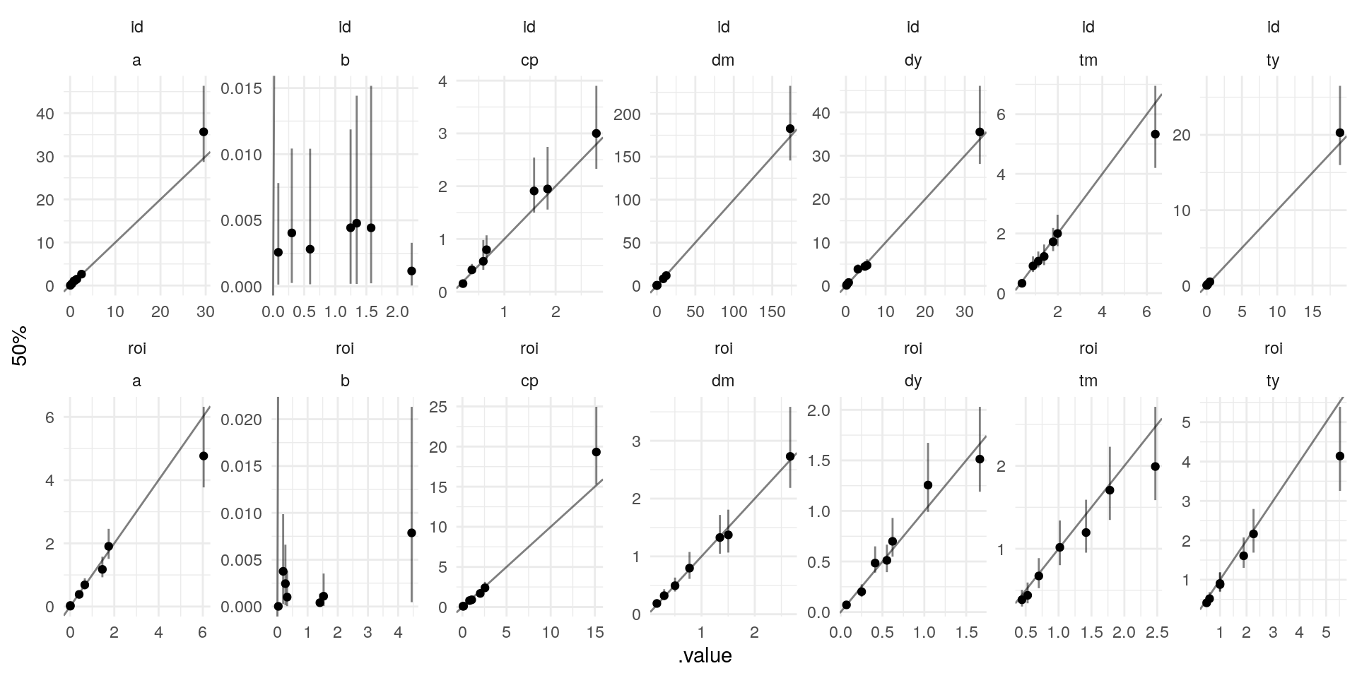
And for your convenience, the plots of the ROI-varying parameters V (they’re similar to the ID-varying U) from all 7 chains. The X axis is the generating value, and the Y axis conveys the posterior where points are medians, and lines are 95% credible intervals (and an identity line in solid black):

And plots of Tau for both V and U:

It does really look like the b parameter is consistently evincing this pathology.

[mike-lawrence]

Hm, maybe @bbbales2 might have some insight?

@mike-lawrence

Just to summarize:

So you have two outcome variables, Y & M , and, in addition to modelling the effect of a few predictors on both, you’re also modelling the influence of M on Y . You have two variables, id and roi that cause variability in the influence of M on Y that you’re modelling hierarchically, and when you simulate data with moderate variability induced by these variables (x-axis of your plots), the posterior for these seem to have much lower variability than expected (y-axis of your plots). And the posterior distribution for the variability parameters, Tau_id[3] and 'Tau_roi[3]` concentrate on very low values.

[bbbales2]

My guess is a non-identifiability in these terms:

U[id, i] + V[roi, i]

where i is 1 to 7 or whatever. This is the new part of the model, right? There used to only be one of these?

Can you make pairplots of them?