Slow sampling fitting an auction model

Slow sampling fitting an auction model


Hi all,

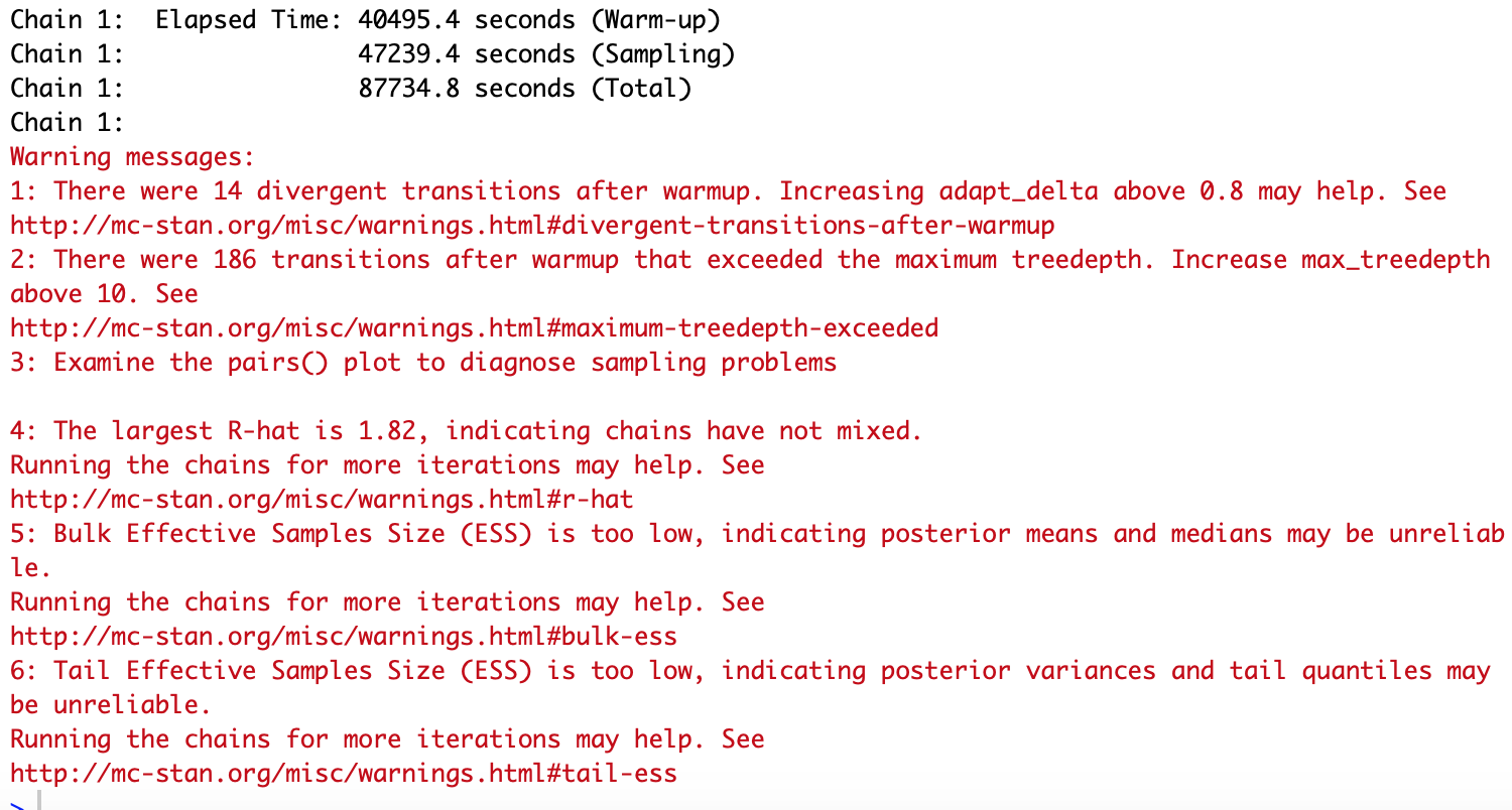
I am working on an auction model and the sampling process in Stan is very slow. It took my laptop over 19 hours to fit 4 MCMC chains with 200 iterations for each. Moreover, all transitions after warm up exceeded the maximum treedepth. I’m wondering whether the usage of integral in the modeling dramatically slow down the sampling or not. If yes, how to improve the performance. Otherwise, what can be the potential problem that slow down the sampling.

The auction model I am working on, in brief, models the bid b_{i} of bidder i by the vector of explanatory variables X_i, the number of competitors J_i -1, and the cost c_{i} through

b_i = c_i + \frac{\int_{c_i}^{\bar{c}} [1-\mbox{F}(c; X_i^\top\beta, \sigma^2)]^{J_i - 1} dc}{[1-\mbox{F}(c_i; X_i\beta, \sigma^2)]^{J_i - 1}} + \epsilon_i\;,\; \epsilon_i \sim \mbox{N}(0, 1)\;,

where \mbox{F}(c; X_i^\top\beta, \sigma) is the cdf of a truncated lognormal distribution \mbox{lognormal}(X_i\beta, \sigma^2)\mbox{T}[0, \bar{c}] defined with hyperparameters \beta, \sigma^2 and the upper bound \bar{c}. The cost c_i is hierarcially modeled by the truncated lognormal distribution

c_i \sim \mbox{lognormal}(X_i\beta, \sigma^2)\mbox{T}[0, \bar{c}]\;.

The target is to obtain the posterior inference of cost c_i for all bidders and hyperparameters \beta and \sigma.

The following lists the parameter and model blocks in Stan code. The complete Stan code is in “generative_model.stan” generative_model.stan (3.0 KB) . One can reproduce the simulation by running “auction_proj.R”.auction_proj.R (1.3 KB) , which calls data.R (3.6 KB) to generate data.

parameters {
  vector[K] beta;
  real<lower=0> sigma;
  vector<lower=0, upper = c_max>[N] costs;
}

model {
  vector[N] inv_hazards;
  
  // priors
  to_vector(beta) ~ normal(0,1);
  sigma ~ normal(1,0.01);
  
  for(i in 1:N){
    costs[i] ~ lognormal(X[i] * beta, sigma) T[,c_max]; //dgp cost distribution
  }
  
  // likelihood
  inv_hazards = getGenerativeTotalAuctionHazard(
                           N,
                           J, // num bidders in each auction
                           costs,
                           X,
                           beta,
                           sigma,
                           c_max,
                           x_r
                           );                        
  (bids - costs) ~ normal(inv_hazards , 1);

}


Thanks,

Lu Zhang


data.R (3.6 KB) auction_proj.R (1.3 KB) generative_model.stan (3.0 KB)

1 Like

@charlesm93 @bgoodri might you have a few mins to take a look/have any ideas for things to try?

Update, fixed a bug in attachment data.R

The model is likely slow because of the large treedepth. I’m guessing your posterior geometry is relatively flat, so your chain “particle” is given a shove, but never makes a U-turn. Moreover, your model may not be very identifiable, either because your data does not inform your parameters or something is degenerate. Can you share some pairs plot?

Just lookin at the code it’s hard to tell what might be going wrong. I’m not sure if your super tight prior on sigma causes issue. I’d consider fixing sigma or widening the prior.

I’m not too familiar with integrate_1d, and I’m not sure how well its performance has been tested. Since the bonds of your integral are finite, you should be able to rewrite your integral using an ODE solver.

1 Like

Maybe generate some synthetic data from a model where the integral has a closed form and then substitute that into the model, that would tell you whether or not the problem is caused specifically by the integration.

Hi Charles,

Thank you so much! I couldn’t agree more that the large treedepth is the main reason of the slow sampling. But I doubt this model has a extremely flat posterior geometry. I made up a simulation using the same code except that I replaced the integral with something like c*(1-F)^{J}. I found the sampling for the made-up example was fast. The sampling process for 4 chains with each 1000 iters cost around 200 seconds. Of course, some of the R-hat of the made-up example were large, that probably indicates identifiable problem. But the speed are so different that makes me feel the problem may comes from the integral.

Also, I have tested with different settings, prior with larger variance, prior for the variance of noise, fixing more parameters. All of them are slow. I also tried the marginalized version, i.e., I marginalize out the cost and just focus on the inference of hyperparameters \beta, \sigma. But my model can’t even be initialized at the true value of the parameters.

I think maybe an ODE solver would be helpful. I will have a try and let you know. Thanks again for your help!

1 Like

Yes, I did something like what you mentioned. I made up a simulation using the same code except that I replaced the integral with something like c*(1-F)^{J}. The sampling process for 4 chains with each 1000 iters cost around 200 seconds. That’s also one of the reason why I think the problem might be caused by the integration.

1 Like

Maybe now replace your closed form with the integration of it’s derivative? If that performs extremely slowly then it has to be the integration step.

I don’t know too much about stan’s internals, but I’m not sure it makes sense for calculating an integral to consume that much extra time – unless the integrand is really wild, it’s not that expensive of a computation in 1 dimension and the gradient shouldn’t be much more difficult than evaluating the integral itself since you can move the gradient inside the integral with Leibniz’s rule.

What is the size of \beta? If \beta is an n-vector then I think it would need to evaluate n integrals to get at the gradient so if n is really large maybe it could get pretty slow.

2 Likes

That is a brilliant idea! I just tried it. I replaced

b_i = c_i + c_b(1-F(c_i))^{J - 1} +\epsilon_i

by

b_i = c_i +\int_{c_i}^{\bar{c}} c_b(J-1)(1-F(u))^{J - 2}f(u) du +\epsilon_i

And here is the comparison of the time estimated by stan:


By the way, the length of \beta is 3.

2 Likes

Interesting. I’m not sure about where to go from there tbh. Seems unreasonably slow to me – maybe open another tread on the performance of integration? If the dimension is low, it may be plausible to evaluate the integral offline at the relevant points and then feed that as data to stan and do some interpolation between points – basically a lookup table for the integral? Not sure if that’s a good idea or not. Or maybe reduce the error tolerance for integration?

Hi Charles,
I tried ODE solver and a less informative prior for sigma. Still quite slow.

Best,

Lu Zhang

@Lu.Zhang This confirms our intuition that the issue is (probably) not with with the numerical integrator, rather the model is poorly identified. I’m guessing the posterior distribution is pretty flat and possibly some of the parameters have a non-finite variance, which is why the chains don’t mix.

I’ll take a closer look. Can you share the fit files (either csv or .Rsave)? I’ll use them to look at further diagnostics.

Hi Charles,

Thank you so much! You can find the code for data and model fitting on the bottom of the post. I am trying other auction modeling, so no rush on this one. ^_^

Best,

Lu Zhang

To be honest, I’d rather not redo the whole fit. Please, send me saved outputs, if you have them (ideally, csv files or saved stanfit object in .Rsave format). If you don’t have them, I highly recommend saving your outputs.

If it’s only a result of a poorly identified model, why is the model with numerical integration over 100x slower compared to a model with the integral evaluated in closed form? Have I misinterpreted the earlier example?

Sorry, I only browsed the thread quickly. Maybe “confirming” non-identifiability is a strong word; but with more diagnostics (e.g. pair plots), I can get a better sense of what is going on. Also, I didn’t suggest it was “only” due to non-identifiability.

In the model fitted with the analytical integral, what was \hat R? Were there warning messages, such as exceeded max tree depth? Do both models return the same result, per examination of the posterior samples? Either yes, and there is an issue on top of the numerical integration being slow; or no, in which case the result of the numerical integral differs from the result of the analytical one – and something gets “lost in translation”.

Hi Charles,

I didn’t save the output so I rerun the project for 500 iterations. I will send you the .RData file of the project through email. The modeling fitting result is saved in “estimated_generative_model”. The fitting took around 5.7 hours. There are a couple of changes I made in the code. I modified the design matrix and the priors for beta and sigma, and I ran the whole project with my old mac. (My linux machine didn’t work after I updated rstan and I am still fixing it T_T). I forgot to screenshot the warning messages but I remember there was a warning about the low tail SSE and the warning message was better than last time. The average treedepth and n_leapfrogs for all chains, as I checked with shinystan, are 5 and 31, respectively.

Best,
Lu Zhang

@charlesm93 @RJTK
Hi all,

Thank you so much for following up this topic! I am fitting the integral performance test model and I will post an update under this topic once I have the result. If you are interested in the .RData result of the integral performance test, please send me your email address so that I can email you the .RData file. My email is lu.zhang@ucla.edu. Thank you again for all your help!

Best,

Lu Zhang

Well, actually I didn’t realize the performance has been improved so much after I made small changes until I compared the new results with my old post. I think the major difference I made is the design matrix of the simulated data. I found the design matrix of the original code doesn’t have the column for the intercept, so I took off one column and added a column for intercept. I am pretty sure changing priors for parameters are not helpful with my old code.

@charlesm93 @RJTK Hi Charles and RJTK,

Here are the screenshots of the running time and warning messages of the programs with integral and without integral:

Here are the fitting results of the two programs:

I think this example supports that using integrate can dramatically slow down the sampling process.

Best,

Lu Zhang

1 Like