Setting custom knots with a B-spline (bs = “bs”)

  • Operating System: macOS
  • brms Version: 2.12.0

I’m trying to fit a univariate B-spline with s(bs = “bs”). The example is based on the recent second edition of Statistical Rethinking, Section 4.5.2, model m4.7. [I’m happy to share the original code from the text, if needed. At the moment, I’m inclined to leave it out to avoid clutter.] If I mostly rely on default settings with s(), I can fit the model fine. However, I run into issues when I try to use custom knots. For example, this works:

# load the packages
library(rethinking)
library(brms)

# load the data
data(cherry_blossoms) 
d <- cherry_blossoms

# complete cases on doy
d2 <- d[complete.cases(d$doy), ] 

# fit the model
prior <- c(
  prior(normal(100, 10), class = Intercept),
  prior(normal(0, 10), class = b),
  prior(normal(0, 10), class = sds),
  prior(exponential(1), class = sigma)
)

m4.7 <-
  brm(data = d2,
      family = gaussian,
      doy ~ 1 + s(year, bs = "bs", m = 3),
      prior = prior,
      chains = 4, cores = 4, seed = 4,
      control = list(adapt_delta = .9))

There are still a few divergent transitions, but overall it works. The complications arise when I try to use the 15 custom knots from the text. Here is the naive approach.

# define the knots
num_knots <- 15
knot_list <- quantile(d2$year, probs = seq(from = 0, to = 1, length.out = num_knots))

# fit the model
m4.7 <-
  brm(data = d2,
      family = gaussian,
      doy ~ 1 + s(year, bs = "bs", m = 3),
      knots = list(year = knot_list),
      prior = prior,
      chains = 4, cores = 4, seed = 4,
      control = list(adapt_delta = .9))

This returns: Error in smooth.construct.bs.smooth.spec(object, dk$data, dk$knots) : there should be 14 supplied knots. One attempt to fix this is to set k = 11.

m4.7 <-
  brm(data = d2,
      family = gaussian,
      doy ~ 1 + s(year, bs = "bs", m = 3, k = 11),
      knots = list(year = knot_list),
      prior = prior,
      chains = 4, cores = 4, seed = 4,
      control = list(adapt_delta = .9))

This fails: Error in splineDesign(knots, x, ord, derivs, outer.ok = outer.ok, sparse = sparse) : the 'x' data must be in the range 1269 to 1833 unless you set 'outer.ok = TRUE'

I have fumbled around with 'outer.ok = TRUE' and attempted many other solutions, but at this point it’s clear I’m in over my head. What am I missing?

@ucfagls, would you mind weighing in?

2 Likes

From ?mgcv::smooth.construct.bs.smooth.spec we see that the number of knots in this parameterisation is k + m[1] + 1, which given the default for k is 10 yields the 14. By setting k = 11 you then get the required number of basis functions for the number of knots supplied. But that isn’t actually what you get, and the help page here is not helpful or clear, so you end up with fewer than 15 basis functions from what I can tell.

I the second error is because the data do not lie exactly within the range of the central knots, for some definition of central. From the help page again we see the requirement for the data to be contained within the k - m[1] + 1 = 9 (by default with k = 10) innermost knots. There is no outer.ok argument (this is to splines::splineDesign() and mgcv doesn’t allow that to be passed). Reading ?splines::splineDesign I think the issue here is really just one of translation from the terminology Richard uses to that used by the authors of splines::splineDesign(). In the help for the latter there is a note saying:

Value:

A matrix with ‘length(x)’ rows and ‘length(knots) - ord’ columns.
The i'th row of the matrix contains the coefficients of the
B-splines (or the indicated derivative of the B-splines) defined
by the ‘knot’ vector and evaluated at the i'th value of ‘x’.  Each
B-spline is defined by a set of ‘ord’ successive knots so the
total number of B-splines is ‘length(knots) - ord’.

To make progress therefore I think you want to set k (and provide knots) such that you have 15 inner knots, which would require k = 17 (from 17 - 3 + 1 = 15), specify the 15 inner knots as Richard had them, but also provide outer values beyond the limits of the data (and thence beyond the range of the inner 15 knots). This seems to work by providing m extreme knots before and after the 15 central knots:

knots <- list(year = c(809, 810, 811, unname(knot_list), 2016, 2017, 2018))

## check we can create the basis
smX <- smoothCon(s(year, bs = "bs", k = 17), data = d2, knots = knots)

## fit model in *mgcv* but should also work in brms
m <- gam(doy ~ s(year, bs = "bs", k = 17), data = d2, knots = knots,
         method = "REML")

I haven’t though about or looked at whether the specification of these m * 2 extra “outer” knots has any bearing on the model results or not, but hopefully just getting this to work will allow you to explore other settings.

I should go an read the healp for mgcv’s 'bs' basis again as it wasn’t clear at all that this was how you needed to set up the knots if a user specified them directly and it doesn’t seem consistent with what I ended up having to do. If there’s an inconsistency I’ll suggest changes to Simon.

2 Likes

First, @ucfagls thank you for the thorough and helpful response.

Second, holy smokes these settings are not intuitive.

Third, you’re right. Now I’m at least moving forward. When I follow your example and fit the model with mgcv::gam(), here are my coefficients:

knots <- list(year = c(809, 810, 811, unname(knot_list), 2016, 2017, 2018))

m <- mgcv::gam(doy ~ s(year, bs = "bs", k = 17), data = d2, knots = knots,
               method = "REML")

m$coefficients
(Intercept)   s(year).1   s(year).2   s(year).3   s(year).4   s(year).5   s(year).6   s(year).7 
104.5405079  -2.4890908   0.2323732   3.4301706   1.3261342   0.3711811  -0.2530850   2.7906470 
  s(year).8   s(year).9  s(year).10  s(year).11  s(year).12  s(year).13  s(year).14  s(year).15 
  2.1916163   2.5260772   3.0136948   2.6765554   3.2343769   1.6196724  -2.5997537  -6.3879879 
 s(year).16 
 -8.4103760 

Is it common to have no residual variance? Also, I was expecting 17 basis estimates. Why only 16? This makes me wonder if we’re not specifying the same model as the original. Backing up a bit, perhaps it would help if I do provide McElreath’s code and results. For the sake of completeness, there will be some redundancies with the code from earlier.

# data
library(rethinking) 
data(cherry_blossoms) 
d <- cherry_blossoms precis(d)
d2 <- d[ complete.cases(d$doy) , ] # complete cases on doy

# knots
num_knots <- 15
knot_list <- quantile( d2$year , probs=seq(0,1,length.out=num_knots) )

# splines
library(splines) 
B <- bs(d2$year,
        knots=knot_list[-c(1,num_knots)] , 
        degree=3 , 
        intercept=TRUE )

# fit the model with rethinking::quap()
m4.7 <- quap( 
  alist(
    D ~ dnorm( mu , sigma ) , mu <- a + B %*% w ,
    a ~ dnorm(100,10),
    w ~ dnorm(0,10),
    sigma ~ dexp(1)
  ), 
  data=list( D=d2$doy , B=B ) , 
  start=list( w=rep( 0 , ncol(B) ) ) 
)

# summary
precis(m4.7,depth=2)

That returns:

        mean   sd   5.5%  94.5%
w[1]   -3.02 3.86  -9.19   3.15
w[2]   -0.83 3.87  -7.01   5.36
w[3]   -1.06 3.58  -6.78   4.67
w[4]    4.84 2.88   0.24   9.44
w[5]   -0.84 2.87  -5.43   3.76
w[6]    4.32 2.91  -0.34   8.98
w[7]   -5.32 2.80  -9.79  -0.84
w[8]    7.84 2.80   3.37  12.32
w[9]   -1.00 2.88  -5.60   3.60
w[10]   3.04 2.91  -1.62   7.69
w[11]   4.67 2.89   0.05   9.29
w[12]  -0.15 2.87  -4.74   4.44
w[13]   5.56 2.89   0.95  10.18
w[14]   0.71 3.00  -4.08   5.51
w[15]  -0.80 3.29  -6.07   4.46
w[16]  -6.96 3.38 -12.36  -1.57
w[17]  -7.67 3.22 -12.82  -2.52
a     103.35 2.37  99.56 107.14
sigma   5.88 0.14   5.65   6.11

The first issues is that identifiability constraints have been applied to the B spline basis; without them, one could add a constant to the intercept and subtract the same “value” from the basis and yield the same model, hence there would be infinitely many models. It seems like Richard fitted an intercept (a) plus one in the basis (intercept = TRUE).

We’ll need to fix that in the GAM to get comparable results, and I don’t think this is possible, certainly not easily such that it would work with brm().

The second issue is that in this example Richard is fitting a regression spline and gam() and brm() will want to fit a penalised spline; we should be able to fix that to match using fx = TRUE in the all to s().

This is as close as I can get for an unpenalised spline; we’re still loosing 1 basis function due to the identifiability constraint and I can’t see a way to stop that.

library(rethinking) 
data(cherry_blossoms) 
d <- cherry_blossoms
d2 <- d[ complete.cases(d$doy) , ] # complete cases on doy

# knots
num_knots <- 15
knot_list <- quantile( d2$year , probs=seq(0,1,length.out=num_knots) )
knots <- list(year = c(809, 810, 811, unname(knot_list), 2016, 2017, 2018))

m <- mgcv::gam(doy ~ s(year, bs = "mybs", k = 17, fx = TRUE, by = 1), data = d2, knots = knots,
               method = "REML")

For this example I think you’d be better off creating the b spline basis using bs() as Richard does and work out how to pass that to a formula in brms.

This is one of those situations where the simple spline case isn’t all that useful in general and as such isn’t in the standard software; you’d typically not want to try to fit a model with unidentifiable terms in it, but I guess the priors Richard used allow the model to fit without issue?

The only real solution to this that i can think of is to write a version of smooth.construct.bs.smooth.spec that does whats needed to stop identifiability constraints being applied (adding a matrix C with all zero values that is a single row with as many as the basis dimension) and adjust other features of the model to match that change this has on the basis dimension (it stays at 17 in the example here, not reduced to 16).

1 Like

Hey @ucfagls, thank you for the helpful answer. I apologize for the response lag. After putting this on the shelf for a while, and with the help from Steve Wild, it’s now clear how to make this work with brms. For posterity, I’ll work it out in two ways:

The single-level option

You’re right to bring up the identifiability issue. Happily, even modest priors solve that problem within the Bayesian context.

Load the focal packages and the data.

library(tidyverse)
library(brms)
library(splines)

data(cherry_blossoms, package = "rethinking")
d <- cherry_blossoms
rm(cherry_blossoms)

# drop missing cases
d2 <-
  d %>% 
  drop_na(doy)

Define the knots and the b-splines.

num_knots <- 15
knot_list <- quantile(d2$year, probs = seq(from = 0, to = 1, length.out = num_knots))

B <- bs(d2$year,
        knots = knot_list[-c(1, num_knots)], 
        degree = 3, 
        intercept = TRUE)

Make a new data set which includes B as a matrix column.

d3 <-
  d2 %>% 
  mutate(B = B) 

Fit the model.

b4.8 <- 
  brm(data = d3,
      family = gaussian,
      doy ~ 1 + B,
      prior = c(prior(normal(100, 10), class = Intercept),
                prior(normal(0, 10), class = b),
                prior(exponential(1), class = sigma)),
      iter = 2000, warmup = 1000, chains = 4, cores = 4,
      seed = 4)

Here’s the model summary.

print(b4.8)
Family: gaussian 
  Links: mu = identity; sigma = identity 
Formula: doy ~ 1 + B 
   Data: d3 (Number of observations: 827) 
Samples: 4 chains, each with iter = 2000; warmup = 1000; thin = 1;
         total post-warmup samples = 4000

Population-Level Effects: 
          Estimate Est.Error l-95% CI u-95% CI Rhat Bulk_ESS Tail_ESS
Intercept   103.59      2.49    98.58   108.45 1.01      761     1071
B1           -3.19      3.88   -10.80     4.21 1.00     1591     2435
B2           -1.11      3.92    -8.82     6.62 1.00     1463     1859
B3           -1.27      3.68    -8.58     6.07 1.00     1332     1833
B4            4.56      2.96    -1.13    10.54 1.00     1046     1648
B5           -1.08      2.99    -6.89     4.78 1.00      954     1399
B6            4.03      3.02    -1.86    10.07 1.00     1056     1515
B7           -5.55      2.91   -11.23     0.30 1.00      981     1672
B8            7.57      2.92     1.92    13.29 1.00     1005     1583
B9           -1.22      2.97    -6.90     4.58 1.01     1001     1458
B10           2.79      3.03    -3.17     9.02 1.00     1019     1527
B11           4.42      3.00    -1.49    10.27 1.00     1056     1846
B12          -0.37      2.99    -5.98     5.70 1.00     1013     1551
B13           5.28      2.99    -0.52    11.07 1.00     1024     1768
B14           0.46      3.09    -5.44     6.74 1.00     1036     1712
B15          -1.05      3.37    -7.77     5.59 1.00     1215     2147
B16          -7.25      3.44   -14.01    -0.49 1.00     1287     1936
B17          -7.88      3.26   -14.24    -1.29 1.00     1246     1824

Family Specific Parameters: 
      Estimate Est.Error l-95% CI u-95% CI Rhat Bulk_ESS Tail_ESS
sigma     5.94      0.14     5.67     6.23 1.00     4173     2921

Samples were drawn using sampling(NUTS). For each parameter, Bulk_ESS
and Tail_ESS are effective sample size measures, and Rhat is the potential
scale reduction factor on split chains (at convergence, Rhat = 1).

Make the bottom panel of McElreath’s Figure 4.13 (p. 118).

fitted(b4.8) %>% 
  data.frame() %>% 
  bind_cols(d3) %>% 
  
  ggplot(aes(x = year, y = doy, ymin = Q2.5, ymax = Q97.5)) + 
  geom_hline(yintercept = fixef(b4.8)[1, 1], linetype = 2) +
  geom_point(color = "steelblue") +
  geom_ribbon(alpha = 2/3) +
  labs(x = "year",
       y = "day in year") +
  theme_classic()

The multilevel option

It seems like we can get a pretty close s()-based analogue with a little tweeking. Here’s my attempt.

b4.11 <-
  brm(data = d2,
      family = gaussian,
      doy ~ 1 + s(year, bs = "bs", k = 19),
      prior = c(prior(normal(100, 10), class = Intercept),
                prior(normal(0, 10), class = b),
                prior(student_t(3, 0, 5.9), class = sds),
                prior(exponential(1), class = sigma)),
      iter = 2000, warmup = 1000, chains = 4, cores = 4,
      seed = 4,
      control = list(adapt_delta = .99))

Parameter summary:

posterior_summary(b4.11)[-22, ] %>% round(2)
              Estimate Est.Error   Q2.5  Q97.5
b_Intercept     104.54      0.20 104.14 104.95
bs_syear_1       -0.09      0.33  -0.75   0.57
sds_syear_1       1.31      0.59   0.54   2.80
sigma             5.98      0.15   5.70   6.28
s_syear_1[1]     -1.37      1.67  -5.50   1.02
s_syear_1[2]     -0.38      0.10  -0.60  -0.19
s_syear_1[3]      0.40      0.24  -0.09   0.88
s_syear_1[4]      1.19      0.42   0.40   2.08
s_syear_1[5]      0.78      0.61  -0.43   2.04
s_syear_1[6]      0.11      0.78  -1.38   1.79
s_syear_1[7]      0.48      0.93  -1.36   2.39
s_syear_1[8]      0.33      1.01  -1.59   2.44
s_syear_1[9]      0.95      1.00  -0.96   3.09
s_syear_1[10]    -0.80      0.95  -2.82   1.02
s_syear_1[11]    -0.43      0.92  -2.38   1.33
s_syear_1[12]    -0.20      0.93  -2.08   1.69
s_syear_1[13]     0.57      1.06  -1.33   2.88
s_syear_1[14]     1.04      1.21  -0.92   3.82
s_syear_1[15]    -0.03      1.10  -2.33   2.20
s_syear_1[16]     1.47      1.46  -0.82   4.86
s_syear_1[17]     1.54      1.54  -0.77   5.38

Make the s()-based alternative to the bbottom panel of McElreath’s Figure 4.13.

fitted(b4.11) %>% 
  data.frame() %>% 
  bind_cols(d3) %>% 
  
  ggplot(aes(x = year, y = doy, ymin = Q2.5, ymax = Q97.5)) + 
  geom_hline(yintercept = fixef(b4.11)[1, 1], linetype = 2) +
  geom_point(color = "steelblue") +
  geom_ribbon(alpha = 2/3) +
  labs(x = "year",
       y = "day in year") +
  theme_classic()

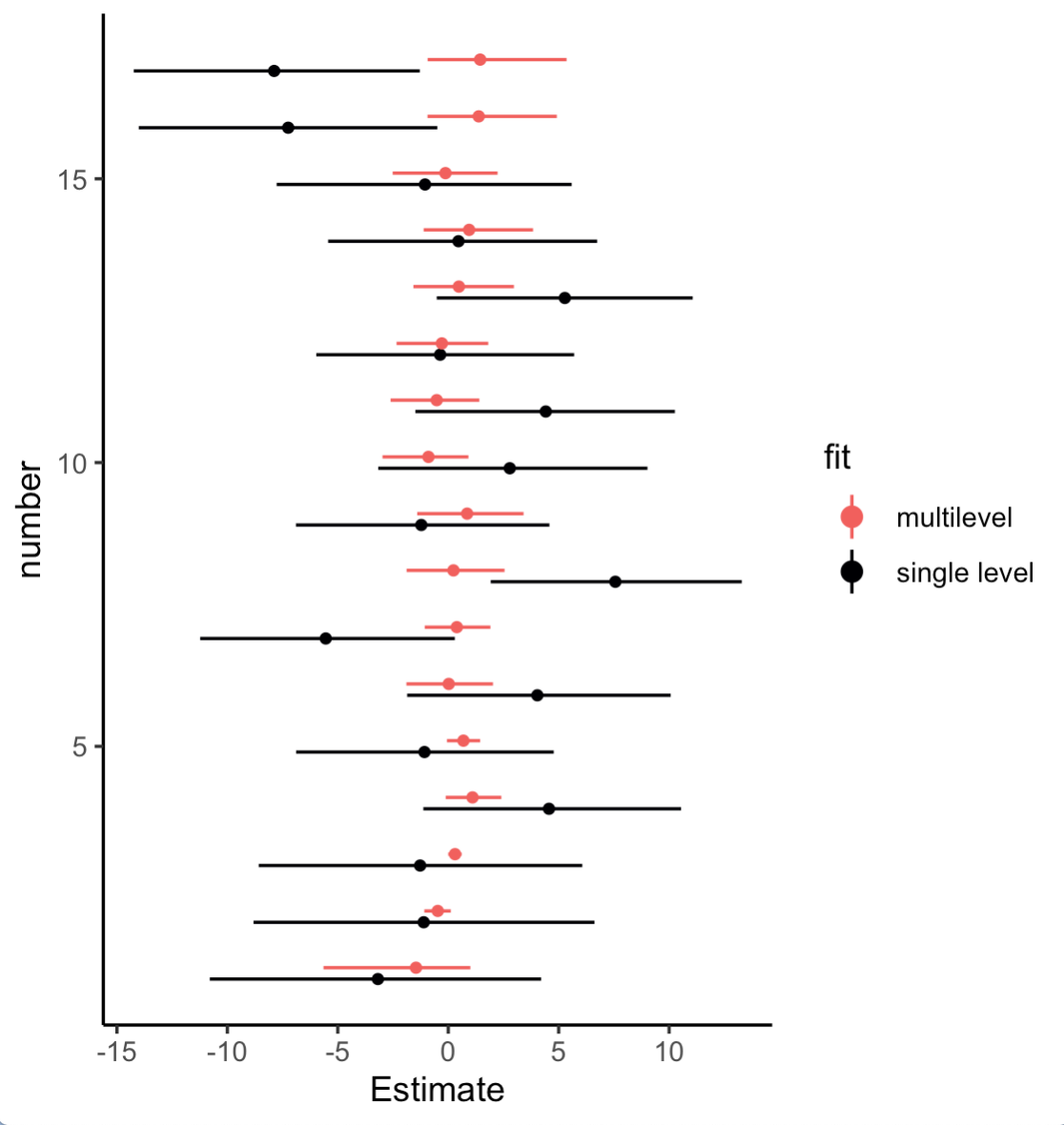
Here we might compare the bias weights from the two models with a coefficient plot.

bind_rows(
  # single level
  fixef(b4.8)[-1, -2] %>% 
    data.frame() %>% 
    mutate(number = 1:n(),
           fit = "single level")  %>% 
    select(fit, number, everything()),
  
  # multilevel (with `s()`)
  posterior_samples(b4.11) %>% 
    select(bs_syear_1, contains("[")) %>% 
    pivot_longer(-bs_syear_1, names_to = "number") %>% 
    mutate(bias = bs_syear_1 + value,
           number = str_remove(number, "s_syear_1") %>% str_extract(., "\\d+") %>% as.integer()) %>% 
    group_by(number) %>% 
    summarise(Estimate = mean(bias),
              Q2.5 = quantile(bias, probs = 0.025),
              Q97.5 = quantile(bias, probs = 0.975)) %>% 
    mutate(fit = "multilevel") %>% 
    select(fit, number, everything())
) %>% 
  mutate(number = if_else(fit == "multilevel", number + 0.1, number - 0.1)) %>% 
  
  # plot
  ggplot(aes(x = Estimate, xmin = Q2.5, xmax = Q97.5, y = number, color = fit)) +
  geom_pointrange(fatten = 1) +
  scale_color_viridis_d(option = "A", end = 2/3, direction = -1) +
  theme_classic()

I’ll be uploading a more detailed walk-out of this workflow in my ebook, soon. In the meantime, the updated code lives on GitHub.

2 Likes