Update
Turns out the error was due to an overrepresentation of values near zero in my MRE. I have slightly altered the MRE and got the model to run:
# generate data
set.seed(10)
x <- as.numeric(0:100)
r <- rnorm(x, mean = 0, sd = ifelse(x == 0, 1, x^-0.8))
c0 <- 2
a <- 0.01
b <- 0.07
k <- 0.05
y <- c0 * exp(-(a * x - b/k * (exp(-k * x) - 1))) + r

require(tidyverse)
require(magrittr)
df <- tibble(x = x, y = y)

stan_code <- "
data {
  int n; // Number of observations
  vector[n] y;    // Response variable
  vector[n] x;    // Predictor variable
}

parameters {
  real<lower=0> sigma; // Standard deviation
  real<lower=0> a;  // Intercept
  real<lower=0> tau; // Precision of random step
  vector[n] k; // Decay rate
}

model {
  // Priors
  sigma ~ exponential( 1 );
  a ~ lognormal( log(2) , 0.05 );
  k[1] ~ lognormal( log(0.08) , 0.05 );
  tau ~ lognormal( log(0.001) , 0.2 );

  // Random walk
  for ( i in 2:n ) {
    k[i] ~ normal( k[i - 1] , tau );
  }

  // Prediction function
  vector[n] mu; // Mean prediction for y
  for( i in 1:n ) {
    mu[i] = a * exp( -k[i] * x[i] ); // Calculate mu using updated k
  }

  // Likelihood
  y ~ normal( mu, sigma );
}
"

# draw samples using RStan
require(rstan)
require(tidybayes)
rw.mod <- stan(model_code = stan_code,
               data = compose_data(df), iter = 2e4,
               chains = 8, cores = parallel::detectCores())

# check Rhat, n_eff and chains
options(max.print = 1e4)
rw.mod
require(rethinking)
trankplot(rw.mod)

# extract prior and posterior distributions
rw.mod.samples <- rw.mod %>%
  spread_draws(sigma, a, tau, k[x]) %>%
  ungroup() %>%
  mutate(
    predictor = rep(df$x, length(unique(.chain)) * length(unique(.iteration))), # recover predictor variable
    sigma_prior = rep(rexp(length(unique(.chain)) * length(unique(.iteration)), 1), # add priors
                      each = length(unique(x))),
    a_prior = rep(rlnorm(length(unique(.chain)) * length(unique(.iteration)), log(2), 0.05),
                  each = length(unique(x))),
    tau_prior = rep(rlnorm(length(unique(.chain)) * length(unique(.iteration)), log(0.001), 0.2),
                    each = length(unique(x))),
    k_prior = rep(rlnorm(length(unique(.chain)) * length(unique(.iteration)), log(0.08), 0.05),
                  each = length(unique(x)))
    )

# prior-posterior comparison
rw.mod.samples %>%
  filter(x == 1) %>%
  pivot_longer(cols = c("sigma", "a", "tau", "k",
                        "sigma_prior", "a_prior", "tau_prior", "k_prior"),
               names_to = c("parameter", "distribution"),
               names_sep = "_",
               values_to = "samples") %>%
  mutate(parameter = fct(parameter),
         distribution = fct(ifelse(is.na(distribution),
                                   "posterior", distribution))) %>%
  ggplot(aes(samples, fill = distribution)) +
    facet_wrap(~parameter, scales = "free", nrow = 1) +
    geom_density(colour = NA, alpha = 0.5) +
    theme_void() +
    theme(legend.position = "top", legend.justification = 0)
The predictions for k (black) do not match the underlying function (orange) perfectly but describe the general trend:
# summarise and plot predictions for k as a function of x
rw.mod.samples %>%
  group_by(predictor) %>%
  summarise(k.mean = mean(k),
            k.pi_lwr50 = PI(k, 0.5)[1],
            k.pi_upr50 = PI(k, 0.5)[2],
            k.pi_lwr80 = PI(k, 0.8)[1],
            k.pi_upr80 = PI(k, 0.8)[2],
            k.pi_lwr90 = PI(k, 0.9)[1],
            k.pi_upr90 = PI(k, 0.9)[2]) %>%
  pivot_longer(cols = starts_with("k.pi"),
               names_to = c("limit", "percentile"),
               names_pattern = ".*_([a-z]+)([0-9]+)") %>%
  pivot_wider(names_from = "limit", values_from = "value") %>%
  ggplot(aes(x = predictor, y = k.mean, ymin = lwr, ymax = upr,
             alpha = percentile)) +
    geom_line() +
    geom_ribbon() +
    stat_function(fun = function(x) { a + b * exp( -k * x ) },
                  colour = "orange") +
    scale_alpha_manual(values = c(0.5, 0.4, 0.3), guide = "none") +
    lims(y = c(0, NA)) +
    theme_minimal()
The predictions for
mu (black) nonetheless fit the data better than the underlying function (orange):
# summarise and plot predictions for mu
rw.mod.samples %>%
  mutate(mu = a * exp( -k * predictor )) %>%
  group_by(predictor) %>%
  summarise(mu.mean = mean(mu),
            mu.pi_lwr50 = PI(mu, 0.5)[1],
            mu.pi_upr50 = PI(mu, 0.5)[2],
            mu.pi_lwr80 = PI(mu, 0.8)[1],
            mu.pi_upr80 = PI(mu, 0.8)[2],
            mu.pi_lwr90 = PI(mu, 0.9)[1],
            mu.pi_upr90 = PI(mu, 0.9)[2]) %>%
  pivot_longer(cols = starts_with("mu.pi"),
               names_to = c("limit", "percentile"),
               names_pattern = ".*_([a-z]+)([0-9]+)") %>%
  pivot_wider(names_from = "limit", values_from = "value") %>%
  ggplot(aes(x = predictor, y = mu.mean)) +
    geom_line() +
    geom_ribbon(aes(ymin = lwr, ymax = upr, alpha = percentile)) +
    stat_function(fun = function(x) { c0 * exp(-(a * x - b/k * (exp(-k * x) - 1))) },
                  colour = "orange") +
    scale_alpha_manual(values = c(0.5, 0.4, 0.3), guide = "none") +
    geom_point(data = df, aes(x, y)) +
    theme_minimal()
With the issue of getting the model to run solved, I focussed my attention on emulating the term
delta in the LibBi function
sub transition. This term defines the step size of the random walk. Stan doesn’t allow decimalised sequences in for loops and the number of steps seems to be limited to
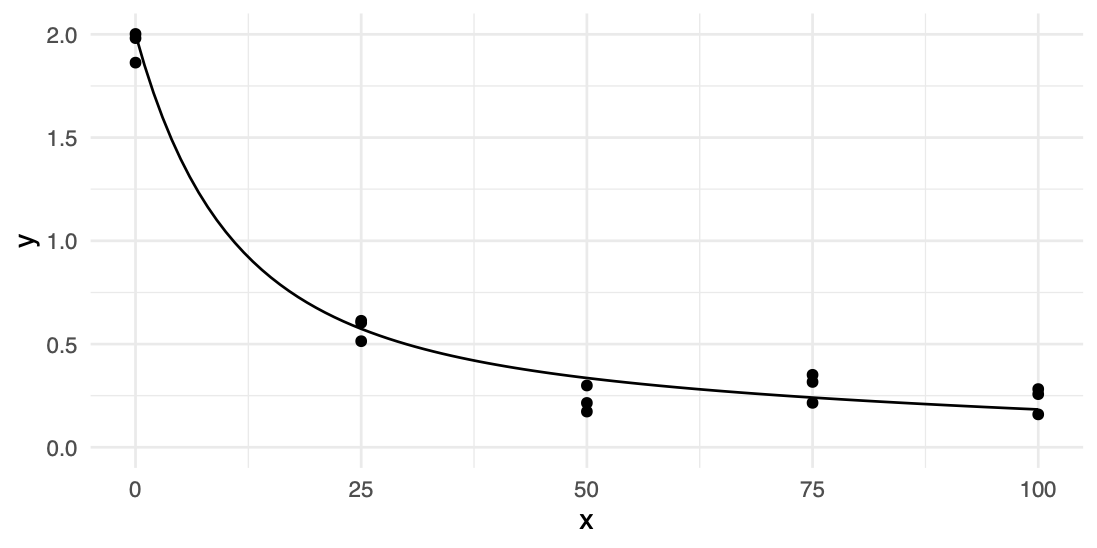
n. A more realistic MRE with gaps in the data provides a case in point:
# generate data with gaps
set.seed(10)
x <- rep(seq(0, 100, 25), each = 3)
r <- rnorm(x, mean = 0, sd = 0.1)
c0 <- 2
a <- 0.01
b <- 0.07
k <- 0.05
y <- c0 * exp(-(a * x - b/k * (exp(-k * x) - 1))) + r

require(tidyverse)
require(magrittr)
df <- tibble(x = x, y = y)

# plot data with underlying function
ggplot(df, aes(x, y)) +
  geom_point() +
  stat_function(fun = function(x) { c0 * exp(-(a * x - b/k * (exp(-k * x) - 1))) }) +
  lims(y = c(0, NA)) +
  theme_minimal()
Since Stan estimates
n steps in
k and
n no longer corresponds directly to
x, it is unclear how to predict the random walk, i.e. interpolate the gaps in the data. However, this is clearly possible as shown in the
paper I initially cited.
@sbfnk, perhaps you can provide some insight into the workings of LibBi’s sub transition(delta = ) and how this may be translated into Stan?