Posterior predictive checks - kurtosis and skew

susanne_s · September 26, 2019, 2:46pm

Operating System: Windows 10
brms Version: 2.9.0

Dear all,

Problem:

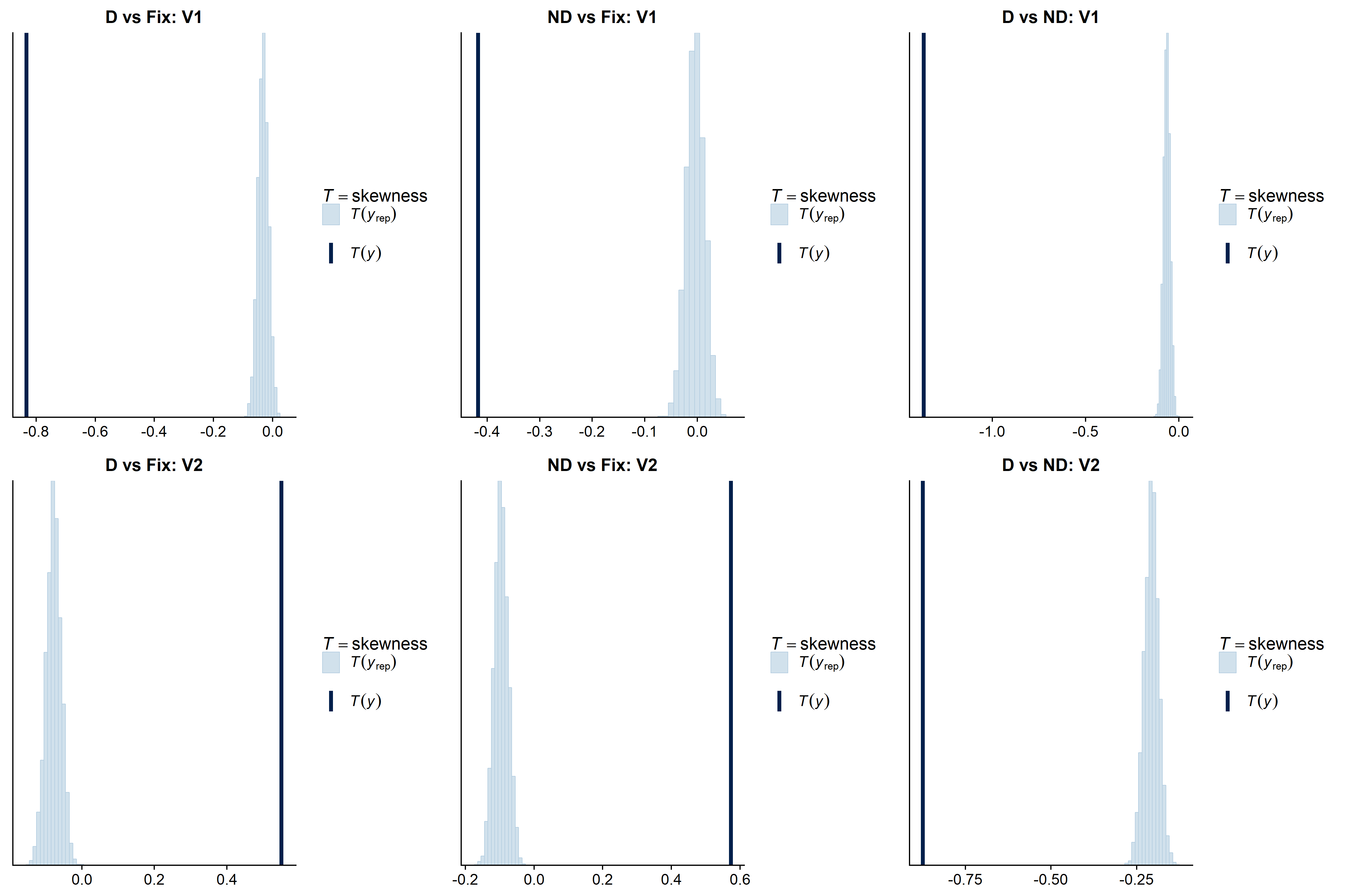
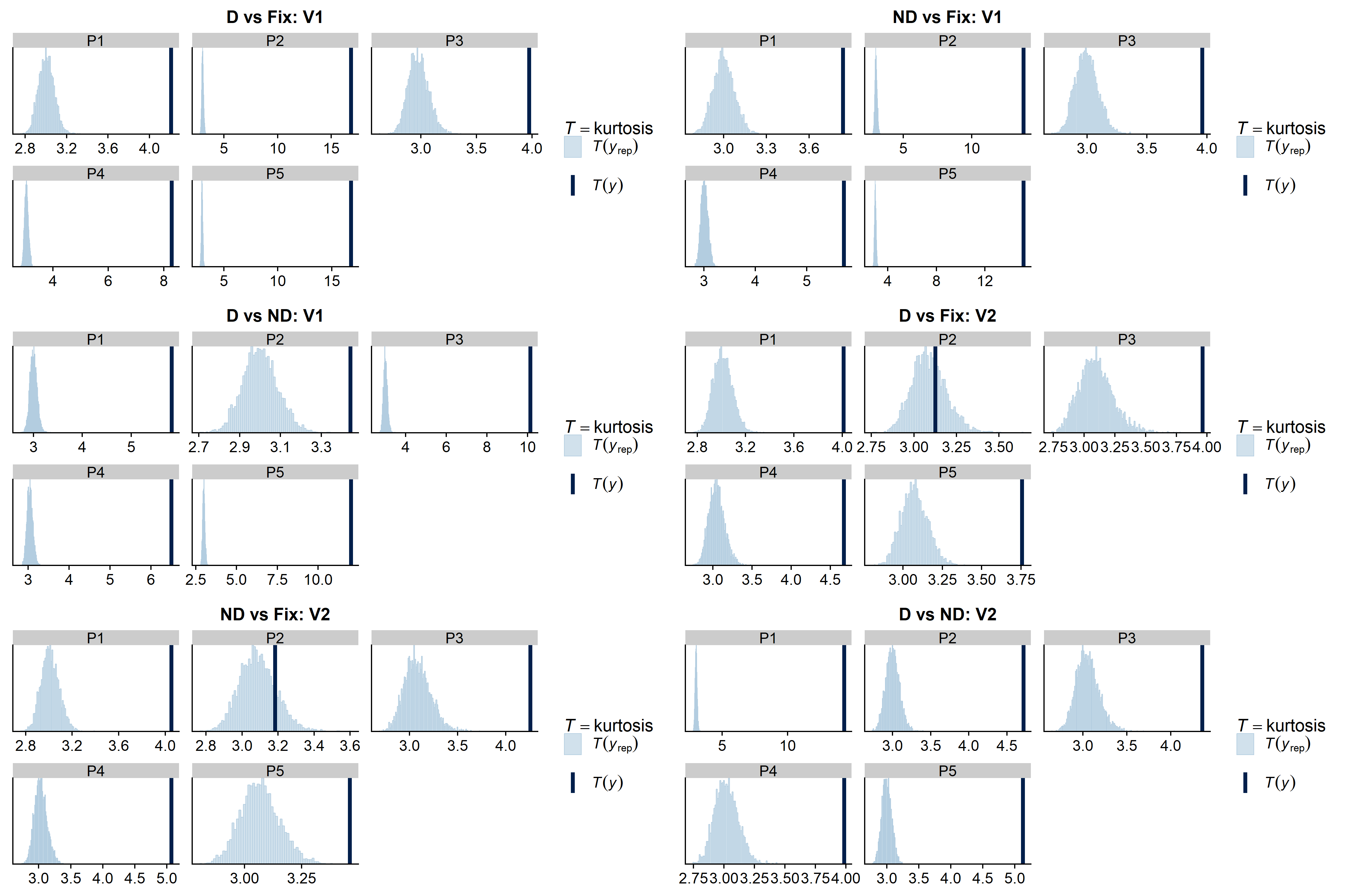
I performed a series of Bayesian MLM analyses on difference scores using brms. I evaluated my models using posterior predictive checks via pp_check(), indicating kurtosis and skew in my data, both of which not captured by my models.
My first impression is that this discrepancy could be potentially tackled by changing the family from Gaussian to sth like (skewed) hyperbolic secant. I might be wrong though.

Questions:

What is your take on this?
How would you tackle these discrepancies?

Posterior predictive checks:

General model details + context:

   Family: gaussian 
  Links: mu = identity; sigma = identity 
Formula: BetaDiff ~ 0 + intercept + VisROI + (1 + VisROI | ID) 
   Data: Data[Data$Contrasts == CurrContrast & Data$Area == (Number of observations: 20381) 
Samples: 4 chains, each with iter = 2000; warmup = 1000; thin = 1;
         total post-warmup samples = 4000

BetaDiff: Differential brain activity
VisROI: Visual field region of interest (i.e. a particular subregion of the visual field); categorical with 4 levels: segments, corners, background, center; dummy-coded with “segments” as a reference category
ID: Participant ID with 5 levels corresponding to 5 human observers
The number of data points for each observer per level of VisROI is at minimum 10 but can be as much as ~3600
The above model specs were used to fit 6 models, one for each contrast of interest (i.e. D vs Fix, ND vs Fix, D vs ND) and brain area (i.e., V1, V2). D and ND reflect different precepts of a visual stimulus and Fix is a fixation baseline where the stimulus was not presented

Priors

> prior_summary(ListFits$ListModels$Segments$`D vs Fix`$V1) 
                  prior class             coef group resp dpar nlpar bound
1                           b                                             
2          normal( 0,7)     b        intercept                            
3          normal( 0,7)     b VisROIBackground                            
4          normal( 0,7)     b     VisROICenter                            
5          normal( 0,7)     b    VisROICorners                            
6  lkj_corr_cholesky(4)     L                                             
7                           L                     ID                      
8          normal(0, 5)    sd                                             
9                          sd                     ID                      
10                         sd        Intercept    ID                      
11                         sd VisROIBackground    ID                      
12                         sd     VisROICenter    ID                      
13                         sd    VisROICorners    ID                      
14         normal(0, 5) sigma                           


> prior_summary(ListFits$ListModels$Segments$`D vs ND`$V1) 
                  prior class             coef group resp dpar nlpar bound
1                           b                                             
2          normal( 0,3)     b        intercept                            
3          normal( 0,3)     b VisROIBackground                            
4          normal( 0,3)     b     VisROICenter                            
5          normal( 0,3)     b    VisROICorners                            
6  lkj_corr_cholesky(4)     L                                             
7                           L                     ID                      
8          normal(0, 5)    sd                                             
9                          sd                     ID                      
10                         sd        Intercept    ID                      
11                         sd VisROIBackground    ID                      
12                         sd     VisROICenter    ID                      
13                         sd    VisROICorners    ID                      
14         normal(0, 5) sigma

The priors for V2 were as for V1 and the priors for ND vs Fix as for D vs Fix
Given that I have only 5 subjects per model, I tightened the default priors on the group-level standard deviations and correlations quite a bit. Please do also note that I ran into problems of divergent transitions with the defaults.

Many thanks in advance for your help!

ldeschamps · September 26, 2019, 3:12pm

Hi!

brms has the skew-normal distribution implemented, you might find it adapted to your problem!

All the best,
Lucas

jonah · September 26, 2019, 10:15pm

Also, if you want to do a PPC that directly checks the skewness you can do something like what we do in Figure 7 of Visualization in Bayesian workflow. The code for making the plot is here

github.com

jgabry/bayes-vis-paper/blob/master/bayes-vis.R#L349-L373


# stat: skew 
skew <- function(x) {
  xdev <- x - mean(x)
  n <- length(x)
  r <- sum(xdev^3) / sum(xdev^2)^1.5
  return(r * sqrt(n) * (1 - 1/n)^1.5)
}


color_scheme_set("blue")
ppc_stat(y, yrep1, stat = "skew", binwidth = 0.01) + 
  xlim(0, .6) + 
  legend_none()
ggsave(filename = "plots/ppc_skew1.png", width = 4.5, height = 3.75)


color_scheme_set("gray")
ppc_stat(y, yrep2, stat = "skew", binwidth = 0.01) + 
  xlim(0, .6) + 
  legend_none()
ggsave(filename = "plots/ppc_skew2.png", width = 4.5, height = 3.75)

This file has been truncated. show original

The code calls the bayesplot package directly but that’s the same package called by pp_check() in brms.

susanne_s · September 27, 2019, 10:05am

Many thanks @ldeschamps! That was indeed one of my first thoughts. Yet, it seems a skewed normal wouldn’t account for the seemingly pronounced leptokurtic properties in e.g. D vs Fix: V1.

susanne_s · September 27, 2019, 10:22am

Many thanks @jonah! I had produced such visualizations already using the package moments. I quickly redid this using your function, leading to negligible differences, so I insert my original plots below.

As you see, skew and kurtosis are not well captured.

Skew

Skew by ID

Kurtosis

Kurtosis by ID

Guido_Biele · September 27, 2019, 10:58am

You could try the student-t distribution to capture the kurtosis.

susanne_s · September 27, 2019, 12:27pm

Up to a point that might be an option. I had been thinking about this a little, but not much, so thank you very much for bringing this up @Guido_Biele! The problem I foresee is that a student-t wouldn’t recover the peakedness being present in some of my graphs.

Besides, having a glimpse at the density plot for D vs ND: V1 (in particular) and the corresponding histograms for skew and kurtosis reveals that I probably need to find a family handling both of these properties at the same time.

So I started thinking about the hyperbolic secant distribution (see e.g. https://arxiv.org/abs/1401.1267) and then (through googling) eventually the generalized skewed hyperbolic secant (see here: https://ideas.repec.org/p/zbw/faucse/462002.html). I have never worked with any of these nor am I currently able to evaluate potential related problems. I therefore appreciate any thoughts on this or related matters very much!

Guido_Biele · September 27, 2019, 12:51pm

About the peaks: I think the student t will do a reasonable way to fit those, but I might be wrong. I would also recommend doing the comparison with histograms instead of density plots (which are derived from the histograms). This should give you a better view on the similarity of y and y_hat.

If the student-t does not capture all aspects of the data that are important to you, you could also try the skewed-t (here is a thread about how to implement it: Skewed distribution).

susanne_s · September 27, 2019, 4:38pm

I wouldn’t think so because as the degrees of freedom go up to infinity, the student distribution becomes gaussian (see e.g. Paul’s vigniette here ftp://ftp.udc.es/CRAN/web/packages/brms/vignettes/brms_families.html) and that’s what I started off with.

I’ll insert below a panel with histograms for y and some yreps. These plots tend to reveal patterns similar to the density plots as far as my eyeballing goes.

Guido_Biele · September 27, 2019, 4:43pm

Are the y-reps for a model with a student t, in which you estimate the degrees of freedom as a parameter?
(I know that the normal distribution is a special case of the student t. My intuition is that if you fit the degrees of freedom as a free parameter, you would estimate low df values, which should allow to capture peaky/fat tailed distributions)

susanne_s · September 30, 2019, 10:30am

No, the yreps are for the original models with a gaussian family.

I would expect the same (to some extent) and maybe I’m underestimating a little what can be recovered. In any case, this is definitely worth a shot and might be a good way of tackling the discrepancies. I set this up now and will report back soonish. Thanks for your input @Guido_Biele !

Guido_Biele · September 30, 2019, 11:17am

no problem,

see also here: https://github.com/stan-dev/math/issues/563 for a short yet clear descripton of how to implement a skew-t by using the t-pdf and t-cdf

susanne_s · October 7, 2019, 3:40pm

Thanks and sorry for not reporting back earlier. I thought I had an epiphany moment, realizing issues in my preprocessing pipeline explaining the leptokurtosis in my data. Yet, as it turns out, I was wrong.

Brief summary

(1) The student-t captured the leptokurtic properties of my data reasonably well as can be seen below; the yrep range is super wide though. In any case, @Guido_Biele, your intuition pumps were well-calibrated! :-)

(2) I then followed @Guido_Biele’s last suggestion and tried to put together a custom skewed student-t based on the provided example. A first attempt + some sensible test results (as far as I can say) can be found below. This is probably riddled with mistakes, so additional pointers/recommendations are of course very welcome.

Posterior predictive checks – student_t – original

Posterior predictive checks – student_t – zoomed-in

Draft - custom skew_student_t

#-----------------------------------------------------------------------------------------
# Skewed student-t - Custom family 
#-----------------------------------------------------------------------------------------

# ........................................................................................ Tidy up 

rm(list = ls())

# ........................................................................................ Seed

set.seed(20191007)

# ........................................................................................ Packages 

library(brms)
library(sn)
library(ggplot2)
library(gridExtra)

# ........................................................................................ Paras

WarmUp    <- 500
Iter      <- 1000
NSamples  <- 10

Extension <- ".png"
XLim      <-  c(-5, 15)
NCol      <- 2
Width     <- 10 
Height    <- 10
Units     <- "in"

# ........................................................................................ Data  

NObs     <- 20000
Sigma    <- 1
Mu       <- 1
Nu       <- 2 
Alpha    <- 2

Data <- data.frame(Response = rst(NObs, xi=Mu, omega = Sigma, alpha=Alpha, nu=Nu))

# ........................................................................................ Custom family 

skew_student_t <- custom_family(
  name = "skew_student_t", dpars = c("mu", "nu","sigma", "alpha"),
  links = "identity", lb = c(NA, 1, 0, NA),
  type = "real")

# Sigma > 0

# ........................................................................................ Stan funcs  

StanFuncs <- "

real skew_student_t_lpdf(real y, real mu, real nu, real sigma, real alpha) {

return log(2) + student_t_lpdf(y | nu, mu, sigma) + student_t_lcdf((y - mu)/sigma * alpha | nu,0, 1);

}


real skew_student_t_rng(real mu, real nu, real sigma, real alpha) {

real z = skew_normal_rng(0, sigma, alpha);
real v = chi_square_rng(nu)/nu;  
real y = mu + z/sqrt(v);

return y;

}

"
# ........................................................................................ Stan vars   

StanVars <- stanvar(scode = StanFuncs, block = "functions")

# ........................................................................................ Fitting  

### Model 
(M0_SkewT <- brm(Response ~ 1, family = skew_student_t, 
                 data = Data, stanvars = StanVars, warmup = WarmUp, iter = Iter))


# Family: skew_student_t 
# Links: mu = identity; nu = identity; sigma = identity; alpha = identity 
# Formula: Response ~ 1 
# Data: Data (Number of observations: 20000) 
# Samples: 4 chains, each with iter = 1000; warmup = 500; thin = 1;
# total post-warmup samples = 2000
# 
# Population-Level Effects: 
#   Estimate Est.Error l-95% CI u-95% CI Eff.Sample Rhat
# Intercept     1.06      0.02     1.02     1.10        522 1.01
# 
# Family Specific Parameters: 
#   Estimate Est.Error l-95% CI u-95% CI Eff.Sample Rhat
# nu        1.83      0.04     1.75     1.90        675 1.00
# sigma     0.92      0.02     0.88     0.96        498 1.01
# alpha     1.99      0.12     1.74     2.24        528 1.01
# 
# Samples were drawn using sampling(NUTS). For each parameter, Eff.Sample 
# is a crude measure of effective sample size, and Rhat is the potential 
# scale reduction factor on split chains (at convergence, Rhat = 1).

### Priors
prior_summary(M0_SkewT)
# prior     class coef group resp dpar nlpar bound
# 1        normal(0, 4)     alpha                                 
# 2 student_t(3, 2, 10) Intercept                                 
# 3       gamma(2, 0.1)        nu                                 
# 4 student_t(3, 0, 10)     sigma   

# ........................................................................................ Expose stan funcs  

expose_functions(M0_SkewT, vectorize = TRUE)

# ........................................................................................ predict   

predict_skew_student_t <- function(i, draws, ...) {
  
  mu    <- draws$dpars$mu[, i]
  sigma <- draws$dpars$sigma
  nu    <- draws$dpars$nu
  alpha <- draws$dpars$alpha
  
  skew_student_t_rng(mu, nu, sigma, alpha)
}

# ........................................................................................ Posterior PC   

PC_Dens_Ori <- pp_check(M0_SkewT, nsamples = NSamples)
PC_Dens_Lim <- PC_Dens_Ori + xlim(XLim)
PC_Hist_Ori <- pp_check(M0_SkewT, type = "hist", nsamples = NSamples, binwidth = 0.1)
PC_Hist_Lim <- PC_Hist_Ori + xlim(XLim)

ListPCPlots <- list(PC_Dens_Ori, PC_Hist_Ori, PC_Dens_Lim, PC_Hist_Lim)
PlotGrid <- grid.arrange(grobs = ListPCPlots,  ncol = NCol) 

ggsave(filename = paste0(quote(M0_SkewT), "_", quote(PlotGrid), Extension), plot = PlotGrid,
       width = Width, height = Height, units = Units)

Posterior predictive checks – custom skew_student_t – original and zoomed-in

susanne_s · October 7, 2019, 3:42pm

Thank you very much @st81 for suggesting this! I will have a look at this.

Guido_Biele · October 8, 2019, 7:24am

Nice that this seems to work.

Unfortunately, I don’t have the time to “review” your code, but here are a few suggestions:

to check if your code works, you can simulate data from the skewed t distribution (https://rdrr.io/cran/sn/man/dst.html) and check if your custom likelihood function allows you to recover the parameters (location, sd, df, skewness).
if you are concerned about the indeed long tails your model produces, you can compare mean, sd, kutosis and skewness of your data and the model predictions. That is, you calculate these parameters for (a) your data and (b) for each iteration for your predicted data. Then you can compare e.g. the true sd and the histogram of sds for the predicted data (I typically plot a histogram of the predicted parameters and use abline to plot the true parameter over the histogram).

In case this is not clear, the idea of the first bullet point is to check if you have a correct implementation of the skewed student-t by using fake data (you could use simulation-based calibration, but I haven’t tried that myself yet). The idea of the second bullet point is to check if your model captures important characteristics of your data by comparing model predictions with your real data.

susanne_s · October 9, 2019, 10:23am

Yeah, quite interesting to see.

Thanks that’s incorporated in my code. The test results are based on fake data.

Thanks. I had a look at some of this already and I am indeed not happy with the long tails, but they might be ok after all.

Thanks for the suggestion. I’ll have a look at simulation-based calibration.

avehtari · October 9, 2019, 10:30am

See also this case study Extreme value analysis and user defined probability functions in Stan
which shows many ways to test user defined distributions.

susanne_s · October 9, 2019, 10:40am

Oh nice; looks super helpful - many thanks!

Guido_Biele · October 9, 2019, 12:27pm

One more thing:
The student-t can be hard to sample* from, so you could try the reparameterization described here: https://mc-stan.org/docs/2_18/stan-users-guide/reparameterization-section.html.
But I am not sure that this helps to deal with the heavy tails in your data.

`* Yes, strictly speaking Stan does not sample, I just don’t know how to say this better ;-)

Topic		Replies	Views
Posterior predictive check looks weird - what can I do? Modeling posterior-predictive , brms	16	3975	April 24, 2024
Plot doesn't look good from pp_check() in brms Modeling brms	3	1066	January 27, 2023
Gaussian vs. skew-normal model selection brms loo	19	7172	August 26, 2019
Choosing family and link brms	24	3711	June 25, 2019
Brms: issues with model specification (gaussian, student) and posterior predictive check Modeling fitting-issues , ecology , brms	1	1035	May 18, 2022

Posterior predictive checks - kurtosis and skew

Related topics