Choosing a sampling distribution for left skewed data

I’m trying to decide on a sampling distribution for a response variable that is left skewed and slightly bimodal. The response variable is fatty acid concentration of tissues, so observed response values are continuous, and positive.

When I fit a simple intercept model with family = gaussian(link=“identity”), pp_check() indicates negative posterior predictions for the response, which doesn’t make biological sense.

condition_master %>%
  filter(lme == "EBS", 
         !vial_id %in% c("2019-65","2019-67","2019-68","2019-71","2019-66"), 
         maturity != 1) -> ebs.dat

model_normal <- brm(Total_FA_Conc_WWT ~ 1, family = gaussian(link="identity"), data = ebs.dat)

I tried to remedy this by truncating the response, but I’m not entirely sure I understand the implications of doing this, and the potential trade offs of instead using a model that allows for negative posterior predictions. I also looked at skew normal, gamma and lognormal distributions, and compared how well each model captures the range, mean, min and max of the data. I was unable to run a truncated skew normal model, as it appeared that predictions could not be evaluated properly at the lower end, leading to NA’s.

# fitting a test brms model with a Gaussian likelihood - truncating response at 0, else models predict values < 0
  #ie. responses out of bounds are discarded
model_normal <- brm(Total_FA_Conc_WWT | trunc(lb = 0) ~ 1, family = gaussian(link="identity"), data = ebs.dat)
summary(model_normal)

# fitting a test brms model with a skew normal likelihood
model_skew <- brm(Total_FA_Conc_WWT  ~ 1, family = skew_normal(), data = ebs.dat)
summary(model_skew)
#If bounded- predictions cannot be evaluated properly at the lower bound, leading to NAs?
#If not bounded, negative posterior predictions for response

# fitting a test brms model with a gamma likelihood
model_gamma <- brm(Total_FA_Conc_WWT ~ 1, family = "gamma", data = ebs.dat)
summary(model_gamma)

# fitting a test brms model with a lognormal likelihood
model_log <- brm(Total_FA_Conc_WWT ~ 1, family = lognormal(), data = ebs.dat)
summary(model_log)

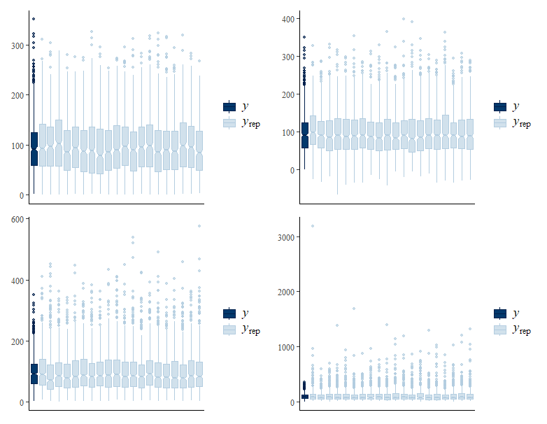
Should have titled, but plots are from top to bottom, L to R: gaussian truncated, skew normal, gamma, and lognormal.

# posterior predictive checking
  pp_check(model_normal, ndraws = 1e2) + pp_check(model_skew, ndraws = 1e2) +
 pp_check(model_gamma, ndraws = 1e2) + pp_check(model_log, ndraws = 1e2) 
#skew normal captures mean and variance best, none of the models picking up apparent bimodality of data 

# posterior predictive checking - boxplots
pp_check(model_normal, type = "boxplot", ndraws = 20) + pp_check(model_skew, type = "boxplot", ndraws = 20) +
  pp_check(model_gamma, type = "boxplot", ndraws = 20) + pp_check(model_log, type = "boxplot", ndraws = 20) 

#and means
pp_check(model_normal, type = "stat", stat = "mean") + pp_check(model_skew, type = "stat", stat = "mean") +
  pp_check(model_gamma, type = "stat", stat = "mean") + pp_check(model_log, type = "stat", stat = "mean")

loo_compare(criterion=“waic”) indicates that predictive accuracy is highest for the gaussian truncated model, but I assume that the skew normal model isn’t top solely because I haven’t effectively truncated the response? Log transforming the raw response doesn’t appear to help much either so I’m uncertain which road to take. How “bad” is bad in regards to posterior predictive checks? And should I just be using family=“gaussian” with truncation given the loo results for my model runs that include covariates?

Windows 10
brms_2.19.0

Also including distribution of minimum and maximum values for posterior distributions

pp_check(model_normal, type = "stat", stat = "min") + pp_check(model_skew, type = "stat", stat = "min") +
  pp_check(model_gamma, type = "stat", stat = "min") + pp_check(model_log, type = "stat", stat = "min")
#skew normal is predicting negative values 

image

#now maximum values
pp_check(model_normal, type = "stat", stat = "max") + pp_check(model_skew, type = "stat", stat = "max") +
    pp_check(model_gamma, type = "stat", stat = "max") + pp_check(model_log, type = "stat", stat = "max")
#lognormal is way overshooting max 

image

Hello @Erin_Fedewa_NOAA_Federal, I suspect that for a positively constrained variable like concentration, your model will need to include some structural constraint to prevent negative predictions, because as you say the normal response model will predict negative concentrations, so the normal and skewnormal response distributions are probably unreasonable at face-value. If the concentration is in fact left-skewed, then I suppose that the major weakness of lognormal or gamma response models will be the right-skew of the distribution, which seems apparent in the PPC. Left-skewed distributions for biologic concentrations are fairly unusual. What does this variable actually look like (say on the log scale)? Might a flexible distribution like the skewnormal on the log-tranformed responses be an option? Personally I would probably take this approach rather than truncation.

A side point is that I presume you will want to work with some covariates here; is it feasible that the left skew of the distribution is explainable by a major covariate?

  • The common terminology would say that your data are right skewed (see Skewness - Wikipedia)
  • Have you used loo() and loo_compare() to check which is providing the best predictions?
  • I recommend to use also pit_ecdf plots.
  • Can you post a reproducible example of failure with truncated skew normal? I think this is something that should work, but may require some changes in the code to make it more robust
  • Eye balling the current plots, the skew normal looks the best, so getting that truncated skew normal would be useful. You could also test skew normal for log(y)
2 Likes

Thank you for the advice!

This is the response variable on log scale:
ebs.dat %>% ggplot(aes(log(Total_FA_Conc_WWT))) + geom_density()
image
I went ahead and tried skew normal on the log-transformed response and the PPC plots definately look much better, so maybe I’ll go that route

#skew normal with log response 
model_skew_log <- brm(log(Total_FA_Conc_WWT)  ~ 1, family = skew_normal(), data = ebs.dat)

image

I had also had the same thought about a covariate explaining the skewed distribution, and imagine that would be very probable. I’ll play around with some model runs including covariates as well, and reassess the PPC plots

The truncated skew normal model runs fine, I just get a warning for NAs being excluded from the model. I also can’t run pp_check() on this model, I assume due to the NAs?

#Bounded skew normal 
model_skew_bound <- brm(Total_FA_Conc_WWT | trunc(lb = 0)  ~ 1, family = skew_normal(), data = ebs.dat)
#If bounded- predictions cannot be evaluated properly at the lower bound, leading to NAs?

Warning message:
Rows containing NAs were excluded from the model.

> pp_check(model_skew_bound, ndraws = 1e2)
Error in `validate_predictions()`:
! NAs not allowed in predictions.
Run `rlang::last_trace()` to see where the error occurred.
There were 50 or more warnings (use warnings() to see the first 50)
> 

Re. my response to @AWoodward, maybe I should pursue log transformation of the response, and the skew normal distribution instead of truncation? I used loo_compare() on the truncated Gaussian, skew normal, gamma and lognormal, and the gaussian truncated had the highest predictive accuracy, but I assume that’s because the skew normal model was predicting negative response values. I assume I can’t use loo to compare a truncated vrs a log-response model because the response variables differ? (see script below). I will look into pit_ecdf plots, that’s a new one for me but thank you for the suggestion!

>   loo_compare(model_normal, model_skew, model_skew_log, model_gamma, model_log, criterion = "waic")
                          elpd_diff se_diff
model_skew_log     0.0       0.0
model_normal   -2142.4      20.3
model_skew     -2153.5      16.7
model_gamma    -2153.8      17.7
model_log      -2217.2      18.0
Warning message:
Not all models have the same y variable. ('yhash' attributes do not match) 
> 

Strange.

You can if you take into account the Jacobian transformation. There is an example of that in Regression and Other Stories chapter 12, with code at Regression and Other Stories: Mesquite.

Thanks for the helpful example @avehtari. I used the Jacobian transformation for Gaussian log(y) and skew normal log(y) models, and then ran loo_compare to assess the Gaussian log(y), skew normal log(y), Gaussian truncated, and skew normal truncated. I’m still trying to sort out what’s going on with the truncated skew normal model, and am not even able to run loo() for it

> loo_skew_trunc <- loo(model_skew_bound)
Error in if (varx == 0) { : missing value where TRUE/FALSE needed
In addition: There were 50 or more warnings (use warnings() to see the first 50)

I dropped the skew normal truncated model from loo_compare() because of this, and the skew normal log(y) model comes out on top.


If I use the skew normal distribution with a log transformed response, should I be worried that my PPC plot (below) still doesn’t look great? I’ll continue to assess once I run more complex models with covariates, and maybe these added covariates will help explain the underlying distribution of the data.

I think the dens_overlay plot for skew normal looks better than for skew normal log. It would be good to get the truncated model to work, and I could have a look, but a reproducible example would help.

I now realized that your formula had ~ 1, so that you didn’t have any covariates. If you do have covariates, they can change completely which distribution is best describing the conditional distribution.

Sorry, forgot to attach the data on my last reply for a reproducible example!
total_FA_master.csv (286.9 KB)

#data wrangling 
condition_master <- read.csv("./data/total_FA_master.csv")

condition_master %>%
 mutate(julian=yday(parse_date_time(start_date, "mdy", "US/Alaska"))) %>%  #add julian date 
 filter(lme == "EBS", 
        !vial_id %in% c("2019-65","2019-67","2019-68","2019-71","2019-66"), 
        maturity != 1) %>%
 mutate(year = as.factor(year),
        sex = as.factor(sex),
        region = as.factor(sample_region),
        station = as.factor(gis_station),
        temperature = as.numeric(gear_temperature),
        fourth.root.cpue = as.numeric(cpue^0.25),
        fourth.root.invert = as.numeric(total_benthic_cpue^0.25)) -> ebs.dat

I was just starting to explore covariate structure and more complex model runs, so as a first pass, I ran a skew normal model that includes two population-level covariates and a group-level effect to explain the spatial structure of the sampling design.

mod5_formula <-  bf(Total_FA_Conc_WWT  ~ cw + s(temperature, k=4)  + (1 | region)) 

mod5 <- brm(mod5_formula,
            data = ebs.dat,
            family = skew_normal(),
            cores = 4, chains = 4, iter = 2500,
            save_pars = save_pars(all = TRUE),
            control = list(adapt_delta = 0.999, max_treedepth = 14))

I had one divergent transition after warmup, and the PPC plot actually looks pretty good. But still predicting negative response values, so maybe a skew normal truncated model is the best way to go moving forward.


Thanks for the example. I can replicate the error. I’ll investigate this.

Thank you!!

should be fixed in the github version of brms.

2 Likes

@paul.buerkner @avehtari I installed the github version of brms and the truncated skew normal distribution model looks good. pp_check() and loo_compare() are running, and are pretty convincing that truncated skew normal is probably the best option for the dataset moving forward, though I will reassess as I add covariates. Thank you for all the assistance, greatly appreciated!
image

@paul.buerkner @avehtari but as a quick follow up to this, it seems that you cannot yet compute posterior draws of the posterior predictive distribution for truncated skew normal models?

> preds <- posterior_epred(mod5) #posterior draws
Error: posterior_epred values on the respone scale not yet implemented for truncated 'skew_normal' models.

Yes, that is what the error message says. There seem to be equations for moments of (at least some version of) skew-normal, so it would be possible to implement this, but I guess @paul.buerkner just didn’t have time and no-one else has asked before.

Meanwhile, maybe posterior_linpred(., transform = TRUE) would be useful? It’s not giving the draws for expectation, but the draws of location parameter. If you need epred, you could use posterior_linpred(., transform = TRUE) and posterior draws of other skew-normal parameters to compute the expectation for each draw yourself using the equations you can find via search engines. If you are not in a hurry, I guess this will get in brms eventually