Hi, I’ve found the problem. The censoring scheme you have used based on only interval censoring is an approximation that introduced the bias that you saw in your posterior predictive check, especially for the example with low mean for the beta part. When the beta part has a low mean, a lot of very low y-values will be generated. In your code, y-values < 0.06 were passed to the model as interval censored data [0.01 - 0.06]. The model will therefore interpret all values < 0.06 as between 0.01 and 0.06, but a lot of generated y-values were < 0.01. This causes bias. The same applies for data that should have been right censored instead of interval censored.
I updated your code to fix this (uses the same .stan file that you have used). PS: thanks for the trick to convert a cmdstanfit back to a brmsfit object. Very cool!
cens_zi_beta_test_2.R (4.4 KB)
cens_zi_beta_aug.stan (3.1 KB)
library(brms)
#> Loading required package: Rcpp
#> Loading 'brms' package (version 2.22.0). Useful instructions
#> can be found by typing help('brms'). A more detailed introduction
#> to the package is available through vignette('brms_overview').
#>
#> Attaching package: 'brms'
#> The following object is masked from 'package:stats':
#>
#> ar
library(tidyverse)
library(cmdstanr)
#> This is cmdstanr version 0.9.0
#> - CmdStanR documentation and vignettes: mc-stan.org/cmdstanr
#> - CmdStan path: C:/Users/hans_vancalster/.cmdstan/cmdstan-2.36.0
#> - CmdStan version: 2.36.0
# custom ppc function ##########################################################
ppc = function(fit, data, ndraws = 10) {
levels = c("0",
"<= 0.05",
"0.05–0.25",
"> 0.25")
observed = case_when(data$y == 0 ~ levels[1],
data$y <= .05 ~ levels[2],
data$y <= .25 ~ levels[3],
data$y > .25 ~ levels[4])
ypred = posterior_predict(fit, ndraws = ndraws)
bins = function(x) {
case_when(x == 0 ~ levels[1],
x <= 0.05 ~ levels[2],
x <= 0.25 ~ levels[3],
x > 0.25 ~ levels[4])
}
sim_bins = apply(ypred, 1, function(x) table(factor(bins(x),
levels = levels)))
sim_df = as.data.frame(t(sim_bins))
sim_df$draw = 1:nrow(sim_df)
obs_counts = table(factor(observed,
levels = levels))
obs_df = data.frame(Category = names(obs_counts),
Observed = as.numeric(obs_counts))
sim_summary = sim_df %>%
pivot_longer(cols = -draw,
names_to = "Category",
values_to = "Simulated") %>%
group_by(Category) %>%
summarise(mean = mean(Simulated),
lower = quantile(Simulated, 0.05),
upper = quantile(Simulated, 0.95))
plot_df = left_join(obs_df, sim_summary, by = "Category") %>%
mutate(Category = factor(Category, levels = levels))
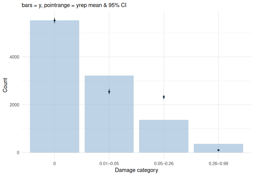
ggplot(plot_df, aes(x = Category)) +
geom_col(aes(y = Observed), fill = "#d0e1eb", alpha = 0.7) +
geom_pointrange(aes(y = mean, ymin = lower, ymax = upper),
color = "#053a6c", size = .25, fatten = 2) +
labs(y = "Count", x = "Damage category",
subtitle = "bars = y, pointrange = yrep mean & 90% CI") +
theme_minimal()
}
# 2. many zeros, lower proportions #############################################
set.seed(123)
n = 1000
x = rnorm(n)
alpha = -2.5
beta = .3
phi = 10
mu = plogis(alpha + beta*x)
alpha_zi = -2.5
beta_zi = -1.5
zi = plogis(alpha_zi + beta_zi*x)
is_zero = rbinom(n, 1, zi)
y = numeric(n)
for (i in 1:n) {
if (is_zero[i] == 1) {
y[i] = 0
} else {
y[i] <- rbeta(1, mu[i] * phi, (1 - mu[i]) * phi)
}
}
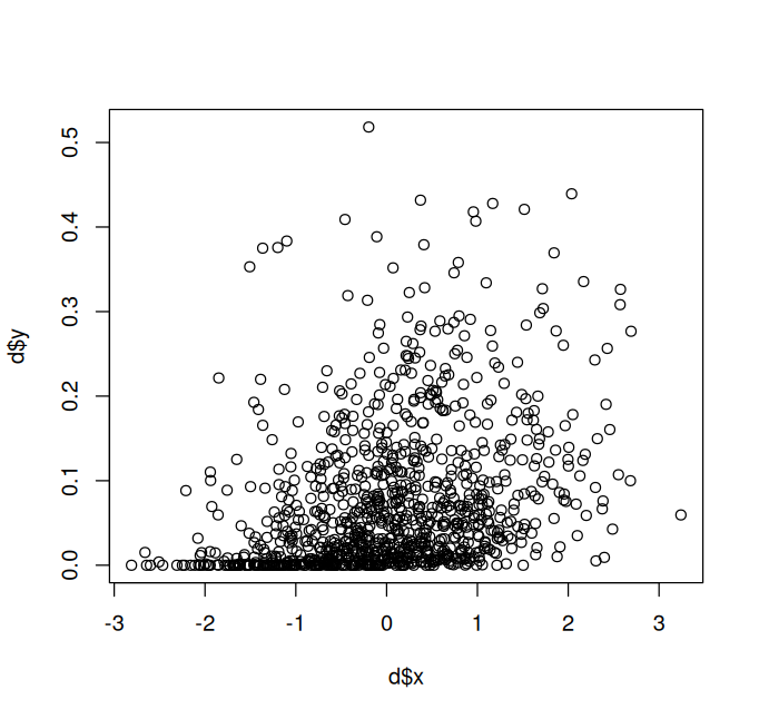
d = data.frame(x = x, y = y)
plot(d$x, d$y)

# with censoring ###########################################################

dcens = d %>%
  mutate(# the lower limits of intervals
    ylow = case_when(y  ==   0 ~ 0,
                     y  <= .05 ~ 1e-7,
                     y  <= .25 ~ .05,
                     y  > .25 ~ .25),
    # the upper limits of intervals
    yhigh = case_when(y  ==   0 ~ 0,
                      y <= .05 ~ .05,
                      y <= .25 ~ .25,
                      y  > .25 ~ 1 - 1e-7),
    # the type of intervals
    censoring = case_when(y  ==   0 ~ "none",
                          y <= .05 ~ "left",
                          y  <= .25 ~ "interval",
                          y  > .25 ~ "right"),
    ycens = case_when(
      censoring == "none" ~ y,
      censoring == "left" ~ yhigh,
      censoring == "right" ~ ylow,
      TRUE ~ ylow
    ))


# modified brms model

formula = bf(
  ycens | cens(censoring, yhigh) ~ x,
  zi ~ x
)
sdata = brms::make_standata(
  formula,
  family = zero_inflated_beta(),
  data = dcens)

model <- cmdstan_model("cens_zi_beta_aug.stan", quiet = TRUE) |>
  suppressMessages()

stanfit <- model$sample(
  data = sdata,
  chains = 4,
  seed = 123,
  parallel_chains = 4
)
#> Running MCMC with 4 parallel chains...
#>
#> Chain 1 Iteration:    1 / 2000 [  0%]  (Warmup)
#> Chain 1 Informational Message: The current Metropolis proposal is about to be rejected because of the following issue:
#> Chain 1 Exception: gamma_lpdf: Random variable is 0, but must be positive finite! (in 'C:/Users/HANS_V~1/AppData/Local/Temp/RtmpOQA2hk/model-347c2f54829.stan', line 82, column 2 to column 41)
#> Chain 1 If this warning occurs sporadically, such as for highly constrained variable types like covariance matrices, then the sampler is fine,
#> Chain 1 but if this warning occurs often then your model may be either severely ill-conditioned or misspecified.
#> Chain 1
#> Chain 1 Informational Message: The current Metropolis proposal is about to be rejected because of the following issue:
#> Chain 1 Exception: Exception: beta_lpdf: First shape parameter is 0, but must be positive finite! (in 'C:/Users/HANS_V~1/AppData/Local/Temp/RtmpOQA2hk/model-347c2f54829.stan', line 8, column 6 to line 9, column 47) (in 'C:/Users/HANS_V~1/AppData/Local/Temp/RtmpOQA2hk/model-347c2f54829.stan', line 100, column 6 to column 71)
#> Chain 1 If this warning occurs sporadically, such as for highly constrained variable types like covariance matrices, then the sampler is fine,
#> Chain 1 but if this warning occurs often then your model may be either severely ill-conditioned or misspecified.
#> Chain 1
#> Chain 1 Informational Message: The current Metropolis proposal is about to be rejected because of the following issue:
#> Chain 1 Exception: gamma_lpdf: Random variable is 0, but must be positive finite! (in 'C:/Users/HANS_V~1/AppData/Local/Temp/RtmpOQA2hk/model-347c2f54829.stan', line 82, column 2 to column 41)
#> Chain 1 If this warning occurs sporadically, such as for highly constrained variable types like covariance matrices, then the sampler is fine,
#> Chain 1 but if this warning occurs often then your model may be either severely ill-conditioned or misspecified.
#> Chain 1
#> Chain 1 Informational Message: The current Metropolis proposal is about to be rejected because of the following issue:
#> Chain 1 Exception: gamma_lpdf: Random variable is 0, but must be positive finite! (in 'C:/Users/HANS_V~1/AppData/Local/Temp/RtmpOQA2hk/model-347c2f54829.stan', line 82, column 2 to column 41)
#> Chain 1 If this warning occurs sporadically, such as for highly constrained variable types like covariance matrices, then the sampler is fine,
#> Chain 1 but if this warning occurs often then your model may be either severely ill-conditioned or misspecified.
#> Chain 1
#> Chain 2 Iteration:    1 / 2000 [  0%]  (Warmup)
#> Chain 2 Informational Message: The current Metropolis proposal is about to be rejected because of the following issue:
#> Chain 2 Exception: gamma_lpdf: Random variable is 0, but must be positive finite! (in 'C:/Users/HANS_V~1/AppData/Local/Temp/RtmpOQA2hk/model-347c2f54829.stan', line 82, column 2 to column 41)
#> Chain 2 If this warning occurs sporadically, such as for highly constrained variable types like covariance matrices, then the sampler is fine,
#> Chain 2 but if this warning occurs often then your model may be either severely ill-conditioned or misspecified.
#> Chain 2
#> Chain 2 Informational Message: The current Metropolis proposal is about to be rejected because of the following issue:
#> Chain 2 Exception: Exception: beta_lpdf: First shape parameter is 0, but must be positive finite! (in 'C:/Users/HANS_V~1/AppData/Local/Temp/RtmpOQA2hk/model-347c2f54829.stan', line 8, column 6 to line 9, column 47) (in 'C:/Users/HANS_V~1/AppData/Local/Temp/RtmpOQA2hk/model-347c2f54829.stan', line 100, column 6 to column 71)
#> Chain 2 If this warning occurs sporadically, such as for highly constrained variable types like covariance matrices, then the sampler is fine,
#> Chain 2 but if this warning occurs often then your model may be either severely ill-conditioned or misspecified.
#> Chain 2
#> Chain 2 Informational Message: The current Metropolis proposal is about to be rejected because of the following issue:
#> Chain 2 Exception: gamma_lpdf: Random variable is inf, but must be positive finite! (in 'C:/Users/HANS_V~1/AppData/Local/Temp/RtmpOQA2hk/model-347c2f54829.stan', line 82, column 2 to column 41)
#> Chain 2 If this warning occurs sporadically, such as for highly constrained variable types like covariance matrices, then the sampler is fine,
#> Chain 2 but if this warning occurs often then your model may be either severely ill-conditioned or misspecified.
#> Chain 2
#> Chain 2 Informational Message: The current Metropolis proposal is about to be rejected because of the following issue:
#> Chain 2 Exception: Exception: beta_lpdf: Second shape parameter is 0, but must be positive finite! (in 'C:/Users/HANS_V~1/AppData/Local/Temp/RtmpOQA2hk/model-347c2f54829.stan', line 8, column 6 to line 9, column 47) (in 'C:/Users/HANS_V~1/AppData/Local/Temp/RtmpOQA2hk/model-347c2f54829.stan', line 100, column 6 to column 71)
#> Chain 2 If this warning occurs sporadically, such as for highly constrained variable types like covariance matrices, then the sampler is fine,
#> Chain 2 but if this warning occurs often then your model may be either severely ill-conditioned or misspecified.
#> Chain 2
#> Chain 3 Iteration:    1 / 2000 [  0%]  (Warmup)
#> Chain 3 Informational Message: The current Metropolis proposal is about to be rejected because of the following issue:
#> Chain 3 Exception: Exception: beta_lpdf: Second shape parameter is 0, but must be positive finite! (in 'C:/Users/HANS_V~1/AppData/Local/Temp/RtmpOQA2hk/model-347c2f54829.stan', line 8, column 6 to line 9, column 47) (in 'C:/Users/HANS_V~1/AppData/Local/Temp/RtmpOQA2hk/model-347c2f54829.stan', line 100, column 6 to column 71)
#> Chain 3 If this warning occurs sporadically, such as for highly constrained variable types like covariance matrices, then the sampler is fine,
#> Chain 3 but if this warning occurs often then your model may be either severely ill-conditioned or misspecified.
#> Chain 3
#> Chain 3 Informational Message: The current Metropolis proposal is about to be rejected because of the following issue:
#> Chain 3 Exception: gamma_lpdf: Random variable is inf, but must be positive finite! (in 'C:/Users/HANS_V~1/AppData/Local/Temp/RtmpOQA2hk/model-347c2f54829.stan', line 82, column 2 to column 41)
#> Chain 3 If this warning occurs sporadically, such as for highly constrained variable types like covariance matrices, then the sampler is fine,
#> Chain 3 but if this warning occurs often then your model may be either severely ill-conditioned or misspecified.
#> Chain 3
#> Chain 4 Iteration:    1 / 2000 [  0%]  (Warmup)
#> Chain 4 Informational Message: The current Metropolis proposal is about to be rejected because of the following issue:
#> Chain 4 Exception: Exception: beta_lpdf: Second shape parameter is 0, but must be positive finite! (in 'C:/Users/HANS_V~1/AppData/Local/Temp/RtmpOQA2hk/model-347c2f54829.stan', line 8, column 6 to line 9, column 47) (in 'C:/Users/HANS_V~1/AppData/Local/Temp/RtmpOQA2hk/model-347c2f54829.stan', line 100, column 6 to column 71)
#> Chain 4 If this warning occurs sporadically, such as for highly constrained variable types like covariance matrices, then the sampler is fine,
#> Chain 4 but if this warning occurs often then your model may be either severely ill-conditioned or misspecified.
#> Chain 4
#> Chain 4 Informational Message: The current Metropolis proposal is about to be rejected because of the following issue:
#> Chain 4 Exception: gamma_lpdf: Random variable is inf, but must be positive finite! (in 'C:/Users/HANS_V~1/AppData/Local/Temp/RtmpOQA2hk/model-347c2f54829.stan', line 82, column 2 to column 41)
#> Chain 4 If this warning occurs sporadically, such as for highly constrained variable types like covariance matrices, then the sampler is fine,
#> Chain 4 but if this warning occurs often then your model may be either severely ill-conditioned or misspecified.
#> Chain 4
#> Chain 4 Informational Message: The current Metropolis proposal is about to be rejected because of the following issue:
#> Chain 4 Exception: Exception: beta_lpdf: Second shape parameter is 0, but must be positive finite! (in 'C:/Users/HANS_V~1/AppData/Local/Temp/RtmpOQA2hk/model-347c2f54829.stan', line 8, column 6 to line 9, column 47) (in 'C:/Users/HANS_V~1/AppData/Local/Temp/RtmpOQA2hk/model-347c2f54829.stan', line 100, column 6 to column 71)
#> Chain 4 If this warning occurs sporadically, such as for highly constrained variable types like covariance matrices, then the sampler is fine,
#> Chain 4 but if this warning occurs often then your model may be either severely ill-conditioned or misspecified.
#> Chain 4
#> Chain 2 Iteration:  100 / 2000 [  5%]  (Warmup)
#> Chain 3 Iteration:  100 / 2000 [  5%]  (Warmup)
#> Chain 1 Iteration:  100 / 2000 [  5%]  (Warmup)
#> Chain 2 Iteration:  200 / 2000 [ 10%]  (Warmup)
#> Chain 4 Iteration:  100 / 2000 [  5%]  (Warmup)
#> Chain 1 Iteration:  200 / 2000 [ 10%]  (Warmup)
#> Chain 2 Iteration:  300 / 2000 [ 15%]  (Warmup)
#> Chain 3 Iteration:  200 / 2000 [ 10%]  (Warmup)
#> Chain 4 Iteration:  200 / 2000 [ 10%]  (Warmup)
#> Chain 1 Iteration:  300 / 2000 [ 15%]  (Warmup)
#> Chain 2 Iteration:  400 / 2000 [ 20%]  (Warmup)
#> Chain 3 Iteration:  300 / 2000 [ 15%]  (Warmup)
#> Chain 1 Iteration:  400 / 2000 [ 20%]  (Warmup)
#> Chain 2 Iteration:  500 / 2000 [ 25%]  (Warmup)
#> Chain 4 Iteration:  300 / 2000 [ 15%]  (Warmup)
#> Chain 3 Iteration:  400 / 2000 [ 20%]  (Warmup)
#> Chain 1 Iteration:  500 / 2000 [ 25%]  (Warmup)
#> Chain 2 Iteration:  600 / 2000 [ 30%]  (Warmup)
#> Chain 3 Iteration:  500 / 2000 [ 25%]  (Warmup)
#> Chain 4 Iteration:  400 / 2000 [ 20%]  (Warmup)
#> Chain 2 Iteration:  700 / 2000 [ 35%]  (Warmup)
#> Chain 1 Iteration:  600 / 2000 [ 30%]  (Warmup)
#> Chain 3 Iteration:  600 / 2000 [ 30%]  (Warmup)
#> Chain 4 Iteration:  500 / 2000 [ 25%]  (Warmup)
#> Chain 1 Iteration:  700 / 2000 [ 35%]  (Warmup)
#> Chain 2 Iteration:  800 / 2000 [ 40%]  (Warmup)
#> Chain 3 Iteration:  700 / 2000 [ 35%]  (Warmup)
#> Chain 4 Iteration:  600 / 2000 [ 30%]  (Warmup)
#> Chain 2 Iteration:  900 / 2000 [ 45%]  (Warmup)
#> Chain 1 Iteration:  800 / 2000 [ 40%]  (Warmup)
#> Chain 3 Iteration:  800 / 2000 [ 40%]  (Warmup)
#> Chain 4 Iteration:  700 / 2000 [ 35%]  (Warmup)
#> Chain 2 Iteration: 1000 / 2000 [ 50%]  (Warmup)
#> Chain 1 Iteration:  900 / 2000 [ 45%]  (Warmup)
#> Chain 2 Iteration: 1001 / 2000 [ 50%]  (Sampling)
#> Chain 3 Iteration:  900 / 2000 [ 45%]  (Warmup)
#> Chain 4 Iteration:  800 / 2000 [ 40%]  (Warmup)
#> Chain 2 Iteration: 1100 / 2000 [ 55%]  (Sampling)
#> Chain 1 Iteration: 1000 / 2000 [ 50%]  (Warmup)
#> Chain 4 Iteration:  900 / 2000 [ 45%]  (Warmup)
#> Chain 1 Iteration: 1001 / 2000 [ 50%]  (Sampling)
#> Chain 3 Iteration: 1000 / 2000 [ 50%]  (Warmup)
#> Chain 3 Iteration: 1001 / 2000 [ 50%]  (Sampling)
#> Chain 2 Iteration: 1200 / 2000 [ 60%]  (Sampling)
#> Chain 3 Iteration: 1100 / 2000 [ 55%]  (Sampling)
#> Chain 1 Iteration: 1100 / 2000 [ 55%]  (Sampling)
#> Chain 4 Iteration: 1000 / 2000 [ 50%]  (Warmup)
#> Chain 4 Iteration: 1001 / 2000 [ 50%]  (Sampling)
#> Chain 2 Iteration: 1300 / 2000 [ 65%]  (Sampling)
#> Chain 3 Iteration: 1200 / 2000 [ 60%]  (Sampling)
#> Chain 2 Iteration: 1400 / 2000 [ 70%]  (Sampling)
#> Chain 1 Iteration: 1200 / 2000 [ 60%]  (Sampling)
#> Chain 4 Iteration: 1100 / 2000 [ 55%]  (Sampling)
#> Chain 3 Iteration: 1300 / 2000 [ 65%]  (Sampling)
#> Chain 2 Iteration: 1500 / 2000 [ 75%]  (Sampling)
#> Chain 3 Iteration: 1400 / 2000 [ 70%]  (Sampling)
#> Chain 4 Iteration: 1200 / 2000 [ 60%]  (Sampling)
#> Chain 1 Iteration: 1300 / 2000 [ 65%]  (Sampling)
#> Chain 2 Iteration: 1600 / 2000 [ 80%]  (Sampling)
#> Chain 3 Iteration: 1500 / 2000 [ 75%]  (Sampling)
#> Chain 2 Iteration: 1700 / 2000 [ 85%]  (Sampling)
#> Chain 3 Iteration: 1600 / 2000 [ 80%]  (Sampling)
#> Chain 4 Iteration: 1300 / 2000 [ 65%]  (Sampling)
#> Chain 1 Iteration: 1400 / 2000 [ 70%]  (Sampling)
#> Chain 2 Iteration: 1800 / 2000 [ 90%]  (Sampling)
#> Chain 3 Iteration: 1700 / 2000 [ 85%]  (Sampling)
#> Chain 4 Iteration: 1400 / 2000 [ 70%]  (Sampling)
#> Chain 2 Iteration: 1900 / 2000 [ 95%]  (Sampling)
#> Chain 1 Iteration: 1500 / 2000 [ 75%]  (Sampling)
#> Chain 3 Iteration: 1800 / 2000 [ 90%]  (Sampling)
#> Chain 2 Iteration: 2000 / 2000 [100%]  (Sampling)
#> Chain 2 finished in 111.7 seconds.
#> Chain 3 Iteration: 1900 / 2000 [ 95%]  (Sampling)
#> Chain 4 Iteration: 1500 / 2000 [ 75%]  (Sampling)
#> Chain 1 Iteration: 1600 / 2000 [ 80%]  (Sampling)
#> Chain 3 Iteration: 2000 / 2000 [100%]  (Sampling)
#> Chain 3 finished in 113.7 seconds.
#> Chain 4 Iteration: 1600 / 2000 [ 80%]  (Sampling)
#> Chain 1 Iteration: 1700 / 2000 [ 85%]  (Sampling)
#> Chain 4 Iteration: 1700 / 2000 [ 85%]  (Sampling)
#> Chain 1 Iteration: 1800 / 2000 [ 90%]  (Sampling)
#> Chain 4 Iteration: 1800 / 2000 [ 90%]  (Sampling)
#> Chain 1 Iteration: 1900 / 2000 [ 95%]  (Sampling)
#> Chain 4 Iteration: 1900 / 2000 [ 95%]  (Sampling)
#> Chain 1 Iteration: 2000 / 2000 [100%]  (Sampling)
#> Chain 1 finished in 122.0 seconds.
#> Chain 4 Iteration: 2000 / 2000 [100%]  (Sampling)
#> Chain 4 finished in 123.3 seconds.
#>
#> All 4 chains finished successfully.
#> Mean chain execution time: 117.7 seconds.
#> Total execution time: 123.5 seconds.

m3b = brm(formula,
          family = zero_inflated_beta(),
          data = dcens, empty = TRUE)
m3b$fit = read_csv_as_stanfit(stanfit$output_files(), model = model)
#> Loading required namespace: rstan
m3b = rename_pars(m3b)
saveRDS(m3b, file = "m3b.rds")
m3b = readRDS("m3b.rds")
summary(m3b)
#>  Family: zero_inflated_beta
#>   Links: mu = logit; phi = identity; zi = logit
#> Formula: ycens | cens(censoring, yhigh) ~ x
#>          zi ~ x
#>    Data: dcens (Number of observations: 1000)
#>   Draws: 4 chains, each with iter = 2000; warmup = 1000; thin = 1;
#>          total post-warmup draws = 4000
#>
#> Regression Coefficients:
#>              Estimate Est.Error l-95% CI u-95% CI Rhat Bulk_ESS Tail_ESS
#> Intercept       -2.46      0.04    -2.54    -2.37 1.00     3060     3247
#> zi_Intercept    -2.61      0.15    -2.93    -2.33 1.00     3522     2618
#> x                0.32      0.04     0.24     0.40 1.00     1876     2986
#> zi_x            -1.45      0.14    -1.73    -1.18 1.00     3435     2943
#>
#> Further Distributional Parameters:
#>     Estimate Est.Error l-95% CI u-95% CI Rhat Bulk_ESS Tail_ESS
#> phi     9.74      0.81     8.24    11.39 1.00     1245     1962
#>
#> Draws were sampled using sample(hmc). For each parameter, Bulk_ESS
#> and Tail_ESS are effective sample size measures, and Rhat is the potential
#> scale reduction factor on split chains (at convergence, Rhat = 1).

ppc(m3b, data = dcens, ndraws = 100)

Created on 2025-07-24 with reprex v2.1.1
Session info
sessioninfo::session_info()
#> Warning in system2("quarto", "-V", stdout = TRUE, env = paste0("TMPDIR=", :
#> running command '"quarto"
#> TMPDIR=C:/Users/hans_vancalster/AppData/Local/Temp/RtmpCQncg7/file3bac25c04088
#> -V' had status 1
#> ─ Session info ───────────────────────────────────────────────────────────────
#>  setting  value
#>  version  R version 4.5.0 (2025-04-11 ucrt)
#>  os       Windows 11 x64 (build 26100)
#>  system   x86_64, mingw32
#>  ui       RTerm
#>  language (EN)
#>  collate  Dutch_Belgium.utf8
#>  ctype    Dutch_Belgium.utf8
#>  tz       Europe/Brussels
#>  date     2025-07-24
#>  pandoc   3.4 @ C:/Program Files/RStudio/resources/app/bin/quarto/bin/tools/ (via rmarkdown)
#>  quarto   NA @ C:\\PROGRA~1\\RStudio\\RESOUR~1\\app\\bin\\quarto\\bin\\quarto.exe
#>
#> ─ Packages ───────────────────────────────────────────────────────────────────
#>  ! package        * version  date (UTC) lib source
#>    abind            1.4-8    2024-09-12 [1] CRAN (R 4.5.0)
#>    backports        1.5.0    2024-05-23 [1] CRAN (R 4.5.0)
#>    bayesplot        1.12.0   2025-04-10 [1] CRAN (R 4.5.0)
#>    bridgesampling   1.1-2    2021-04-16 [1] CRAN (R 4.5.0)
#>    brms           * 2.22.0   2024-09-23 [1] CRAN (R 4.5.0)
#>    Brobdingnag      1.2-9    2022-10-19 [1] CRAN (R 4.5.0)
#>    checkmate        2.3.2    2024-07-29 [1] CRAN (R 4.5.0)
#>    cli              3.6.5    2025-04-23 [1] CRAN (R 4.5.0)
#>    cmdstanr       * 0.9.0    2025-04-27 [1] https://stan-dev.r-universe.dev (R 4.5.0)
#>    coda             0.19-4.1 2024-01-31 [1] CRAN (R 4.5.0)
#>    codetools        0.2-20   2024-03-31 [2] CRAN (R 4.5.0)
#>    curl             6.2.2    2025-03-24 [1] CRAN (R 4.5.0)
#>    data.table       1.17.2   2025-05-12 [1] CRAN (R 4.5.0)
#>    dichromat        2.0-0.1  2022-05-02 [1] CRAN (R 4.5.0)
#>    digest           0.6.37   2024-08-19 [1] CRAN (R 4.5.0)
#>    distributional   0.5.0    2024-09-17 [1] CRAN (R 4.5.0)
#>    dplyr          * 1.1.4    2023-11-17 [1] CRAN (R 4.5.0)
#>    emmeans          1.11.1   2025-05-04 [1] CRAN (R 4.5.0)
#>    estimability     1.5.1    2024-05-12 [1] CRAN (R 4.5.0)
#>    evaluate         1.0.3    2025-01-10 [1] CRAN (R 4.5.0)
#>    farver           2.1.2    2024-05-13 [1] CRAN (R 4.5.0)
#>    fastmap          1.2.0    2024-05-15 [1] CRAN (R 4.5.0)
#>    forcats        * 1.0.0    2023-01-29 [1] CRAN (R 4.5.0)
#>    fs               1.6.6    2025-04-12 [1] CRAN (R 4.5.0)
#>    generics         0.1.4    2025-05-09 [1] CRAN (R 4.5.0)
#>    ggplot2        * 3.5.2    2025-04-09 [1] CRAN (R 4.5.0)
#>    glue             1.8.0    2024-09-30 [1] CRAN (R 4.5.0)
#>    gridExtra        2.3      2017-09-09 [1] CRAN (R 4.5.0)
#>    gtable           0.3.6    2024-10-25 [1] CRAN (R 4.5.0)
#>    hms              1.1.3    2023-03-21 [1] CRAN (R 4.5.0)
#>    htmltools        0.5.8.1  2024-04-04 [1] CRAN (R 4.5.0)
#>    inline           0.3.21   2025-01-09 [1] CRAN (R 4.5.0)
#>    jsonlite         2.0.0    2025-03-27 [1] CRAN (R 4.5.0)
#>    knitr            1.50     2025-03-16 [1] CRAN (R 4.5.0)
#>    labeling         0.4.3    2023-08-29 [1] CRAN (R 4.5.0)
#>    lattice          0.22-7   2025-04-02 [2] CRAN (R 4.5.0)
#>    lifecycle        1.0.4    2023-11-07 [1] CRAN (R 4.5.0)
#>    loo              2.8.0    2024-07-03 [1] CRAN (R 4.5.0)
#>    lubridate      * 1.9.4    2024-12-08 [1] CRAN (R 4.5.0)
#>    magrittr         2.0.3    2022-03-30 [1] CRAN (R 4.5.0)
#>    Matrix           1.7-3    2025-03-11 [2] CRAN (R 4.5.0)
#>    matrixStats      1.5.0    2025-01-07 [1] CRAN (R 4.5.0)
#>    mvtnorm          1.3-3    2025-01-10 [1] CRAN (R 4.5.0)
#>    nlme             3.1-168  2025-03-31 [2] CRAN (R 4.5.0)
#>    pillar           1.10.2   2025-04-05 [1] CRAN (R 4.5.0)
#>    pkgbuild         1.4.7    2025-03-24 [1] CRAN (R 4.5.0)
#>    pkgconfig        2.0.3    2019-09-22 [1] CRAN (R 4.5.0)
#>    plyr             1.8.9    2023-10-02 [1] CRAN (R 4.5.0)
#>    posterior        1.6.1    2025-02-27 [1] CRAN (R 4.5.0)
#>    processx         3.8.6    2025-02-21 [1] CRAN (R 4.5.0)
#>    ps               1.9.1    2025-04-12 [1] CRAN (R 4.5.0)
#>    purrr          * 1.0.4    2025-02-05 [1] CRAN (R 4.5.0)
#>    QuickJSR         1.7.0    2025-03-31 [1] CRAN (R 4.5.0)
#>    R6               2.6.1    2025-02-15 [1] CRAN (R 4.5.0)
#>    RColorBrewer     1.1-3    2022-04-03 [1] CRAN (R 4.5.0)
#>    Rcpp           * 1.0.14   2025-01-12 [1] CRAN (R 4.5.0)
#>  D RcppParallel     5.1.10   2025-01-24 [1] CRAN (R 4.5.0)
#>    readr          * 2.1.5    2024-01-10 [1] CRAN (R 4.5.0)
#>    reprex           2.1.1    2024-07-06 [1] CRAN (R 4.5.0)
#>    reshape2         1.4.4    2020-04-09 [1] CRAN (R 4.5.0)
#>    rlang            1.1.6    2025-04-11 [1] CRAN (R 4.5.0)
#>    rmarkdown        2.29     2024-11-04 [1] CRAN (R 4.5.0)
#>    rstan            2.32.7   2025-03-10 [1] CRAN (R 4.5.0)
#>    rstantools       2.4.0    2024-01-31 [1] CRAN (R 4.5.0)
#>    rstudioapi       0.17.1   2024-10-22 [1] CRAN (R 4.5.0)
#>    scales           1.4.0    2025-04-24 [1] CRAN (R 4.5.0)
#>    sessioninfo      1.2.3    2025-02-05 [1] CRAN (R 4.5.0)
#>    StanHeaders      2.32.10  2024-07-15 [1] CRAN (R 4.5.0)
#>    stringi          1.8.7    2025-03-27 [1] CRAN (R 4.5.0)
#>    stringr        * 1.5.1    2023-11-14 [1] CRAN (R 4.5.0)
#>    tensorA          0.36.2.1 2023-12-13 [1] CRAN (R 4.5.0)
#>    tibble         * 3.2.1    2023-03-20 [1] CRAN (R 4.5.0)
#>    tidyr          * 1.3.1    2024-01-24 [1] CRAN (R 4.5.0)
#>    tidyselect       1.2.1    2024-03-11 [1] CRAN (R 4.5.0)
#>    tidyverse      * 2.0.0    2023-02-22 [1] CRAN (R 4.5.0)
#>    timechange       0.3.0    2024-01-18 [1] CRAN (R 4.5.0)
#>    tzdb             0.5.0    2025-03-15 [1] CRAN (R 4.5.0)
#>    vctrs            0.6.5    2023-12-01 [1] CRAN (R 4.5.0)
#>    withr            3.0.2    2024-10-28 [1] CRAN (R 4.5.0)
#>    xfun             0.52     2025-04-02 [1] CRAN (R 4.5.0)
#>    xml2             1.3.8    2025-03-14 [1] CRAN (R 4.5.0)
#>    xtable           1.8-4    2019-04-21 [1] CRAN (R 4.5.0)
#>    yaml             2.3.10   2024-07-26 [1] CRAN (R 4.5.0)
#>
#>  [1] C:/R/library
#>  [2] C:/R/R-4.5.0/library
#>
#>  * ── Packages attached to the search path.
#>  D ── DLL MD5 mismatch, broken installation.
#>
#> ──────────────────────────────────────────────────────────────────────────────