Here is a reprex:
Data.csv (38.0 KB)
# List of needed packages
Pkgs <- c("tidyverse", "parallel", "cmdstanr",
"brms", "tidybayes", "tidytext")
# Load packages
lapply(Pkgs, require, c = T)
## Set computing options
ncores = detectCores()
# Read in data
Data <- read.csv(file = here("data", "Data.csv")) %>%
mutate(ID = factor(ID),
Group = factor(Group),
Condition = factor(Condition),
Type = factor(Type))
brms model
## brms zero inflated binomial formula
zi_fmla <- bf(Response | trials(1) ~ 1 +
Group +
Condition +
Type +
Condition:Type +
(1 + Condition + Type | ID),
center = FALSE,
zi ~ Type + (1 + Condition + Type | ID)
)
## Set priors
zi_priors <- c(
set_prior("normal(0,1)",
class = "b",
coef = "Intercept"),
set_prior("normal(0,1)",
class = "b"),
set_prior("normal(0,1)",
class = "sd")
)
# Fit model in brms
zi_Mod <- brm(zi_fmla,
Data,
family = zero_inflated_binomial(),
prior = zi_priors,
inits = "random",
iter = 2000,
warmup = 1000,
chains = 4,
cores = ncores,
backend = "cmdstan",
normalize = FALSE,
control = list(adapt_delta = 0.99,
max_treedepth = 14)
)
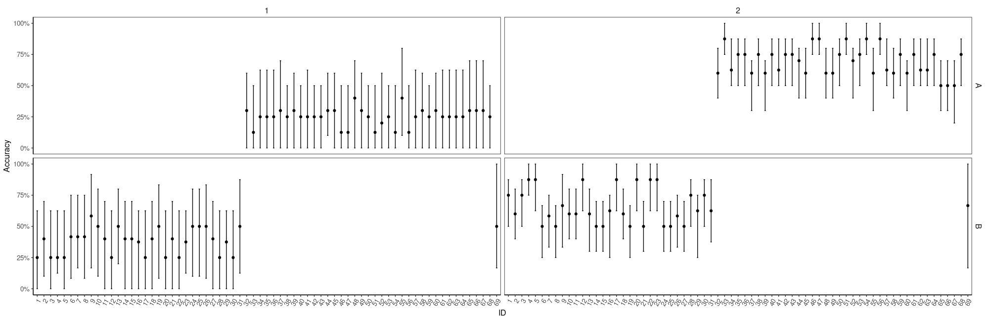
Look at accuracy
Data %>%
add_predicted_draws(zi_Mod,
value = "Pred",
re_formula = NULL) %>%
ungroup() %>%
mutate(Correct = ifelse(Response == Pred, 1, 0)) %>%
group_by(ID, Group, Type, .draw) %>%
summarize(Accuracy = sum(Correct)/n()) %>%
ungroup() %>%
group_by(ID, Group, Type) %>%
point_interval(Accuracy,
.width = 0.89,
.point = median,
.interval = hdci,
.simple_names = TRUE,
na.rm = TRUE) %>%
ungroup() %>%
ggplot(aes(reorder_within(ID, -Accuracy, Group), Accuracy)) +
facet_grid(Group ~ Type, scales = "free_x") +
geom_point(position = position_dodge(width = 0.5)) +
geom_errorbar(aes(
ymin = .lower,
ymax = .upper),
width = 0.2,
position = position_dodge(width = 0.5)) +
scale_x_reordered("ID") +
scale_y_continuous("Accuracy", labels = scales::percent_format(accuracy = 1)) +
theme_bw() +
theme_bw() +
theme(
axis.text.x = element_text(angle = 60, hjust = 1, size = 10),
axis.text.y = element_text(size = 10),
axis.title.x = element_text(size = 12),
axis.title.y = element_text(size = 12),
plot.title = element_text(hjust = 0.5),
panel.border = element_rect(fill = NA, colour = "black"),
panel.grid.major = element_blank(),
panel.grid.minor = element_blank(),
axis.line = element_line(colour = "black"),
strip.text.x = element_text(size = 12),
strip.text.y = element_text(size = 12),
strip.background = element_blank(),
legend.title = element_blank(),
legend.text = element_text(size = 10),
legend.position = c(0.95, 0.05),
legend.key = element_rect(fill = "transparent"),
legend.direction = "horizontal",
legend.background = element_rect(fill = "transparent", size = 6)
)
Now fit the model with Stan code generated by stancode(zi_Mod)
# Model code
Stan_Code <- "functions {
/* compute correlated group-level effects
* Args:
* z: matrix of unscaled group-level effects
* SD: vector of standard deviation parameters
* L: cholesky factor correlation matrix
* Returns:
* matrix of scaled group-level effects
*/
matrix scale_r_cor(matrix z, vector SD, matrix L) {
// r is stored in another dimension order than z
return transpose(diag_pre_multiply(SD, L) * z);
}
/* zero-inflated binomial log-PDF of a single response
   * Args:
   *   y: the response value
   *   trials: number of trials of the binomial part
   *   theta: probability parameter of the binomial part
   *   zi: zero-inflation probability
   * Returns:
   *   a scalar to be added to the log posterior
   */
  real zero_inflated_binomial_lpmf(int y, int trials,
                                   real theta, real zi) {
    if (y == 0) {
      return log_sum_exp(bernoulli_lpmf(1 | zi),
                         bernoulli_lpmf(0 | zi) +
                         binomial_lpmf(0 | trials, theta));
    } else {
      return bernoulli_lpmf(0 | zi) +
             binomial_lpmf(y | trials, theta);
    }
  }
  /* zero-inflated binomial log-PDF of a single response
   * logit parameterization of the zero-inflation part
   * Args:
   *   y: the response value
   *   trials: number of trials of the binomial part
   *   theta: probability parameter of the binomial part
   *   zi: linear predictor for zero-inflation part
   * Returns:
   *   a scalar to be added to the log posterior
   */
  real zero_inflated_binomial_logit_lpmf(int y, int trials,
                                         real theta, real zi) {
    if (y == 0) {
      return log_sum_exp(bernoulli_logit_lpmf(1 | zi),
                         bernoulli_logit_lpmf(0 | zi) +
                         binomial_lpmf(0 | trials, theta));
    } else {
      return bernoulli_logit_lpmf(0 | zi) +
             binomial_lpmf(y | trials, theta);
    }
  }
  /* zero-inflated binomial log-PDF of a single response
   * logit parameterization of the binomial part
   * Args:
   *   y: the response value
   *   trials: number of trials of the binomial part
   *   eta: linear predictor for binomial part
   *   zi: zero-inflation probability
   * Returns:
   *   a scalar to be added to the log posterior
   */
  real zero_inflated_binomial_blogit_lpmf(int y, int trials,
                                          real eta, real zi) {
    if (y == 0) {
      return log_sum_exp(bernoulli_lpmf(1 | zi),
                         bernoulli_lpmf(0 | zi) +
                         binomial_logit_lpmf(0 | trials, eta));
    } else {
      return bernoulli_lpmf(0 | zi) +
             binomial_logit_lpmf(y | trials, eta);
    }
                                          }
  /* zero-inflated binomial log-PDF of a single response
   * logit parameterization of the binomial part
   * logit parameterization of the zero-inflation part
   * Args:
   *   y: the response value
   *   trials: number of trials of the binomial part
   *   eta: linear predictor for binomial part
   *   zi: linear predictor for zero-inflation part
   * Returns:
   *   a scalar to be added to the log posterior
   */
  real zero_inflated_binomial_blogit_logit_lpmf(int y, int trials,
                                                real eta, real zi) {
    if (y == 0) {
      return log_sum_exp(bernoulli_logit_lpmf(1 | zi),
                         bernoulli_logit_lpmf(0 | zi) +
                         binomial_logit_lpmf(0 | trials, eta));
    } else {
      return bernoulli_logit_lpmf(0 | zi) +
             binomial_logit_lpmf(y | trials, eta);
    }
  }
  // zero-inflated binomial log-CCDF and log-CDF functions
  real zero_inflated_binomial_lccdf(int y, int trials, real theta, real zi) {
    return bernoulli_lpmf(0 | zi) + binomial_lccdf(y | trials, theta);
  }
  real zero_inflated_binomial_lcdf(int y, int trials, real theta, real zi) {
    return log1m_exp(zero_inflated_binomial_lccdf(y | trials, theta, zi));
  }
}
data {
int<lower=1> N; // total number of observations
int Y[N]; // response variable
int trials[N]; // number of trials
int<lower=1> K; // number of population-level effects
matrix[N, K] X; // population-level design matrix
int<lower=1> K_zi; // number of population-level effects
matrix[N, K_zi] X_zi; // population-level design matrix
// data for group-level effects of ID 1
int<lower=1> N_1; // number of grouping levels
int<lower=1> M_1; // number of coefficients per level
int<lower=1> J_1[N]; // grouping indicator per observation
// group-level predictor values
vector[N] Z_1_1;
vector[N] Z_1_2;
vector[N] Z_1_3;
int<lower=1> NC_1; // number of group-level correlations
// data for group-level effects of ID 2
int<lower=1> N_2; // number of grouping levels
int<lower=1> M_2; // number of coefficients per level
int<lower=1> J_2[N]; // grouping indicator per observation
// group-level predictor values
vector[N] Z_2_zi_1;
vector[N] Z_2_zi_2;
vector[N] Z_2_zi_3;
int<lower=1> NC_2; // number of group-level correlations
int prior_only; // should the likelihood be ignored?
}
transformed data {
int Kc_zi = K_zi - 1;
matrix[N, Kc_zi] Xc_zi; // centered version of X_zi without an intercept
vector[Kc_zi] means_X_zi; // column means of X_zi before centering
for (i in 2:K_zi) {
means_X_zi[i - 1] = mean(X_zi[, i]);
Xc_zi[, i - 1] = X_zi[, i] - means_X_zi[i - 1];
}
}
parameters {
vector[K] b; // population-level effects
vector[Kc_zi] b_zi; // population-level effects
real Intercept_zi; // temporary intercept for centered predictors
vector<lower=0>[M_1] sd_1; // group-level standard deviations
matrix[M_1, N_1] z_1; // standardized group-level effects
cholesky_factor_corr[M_1] L_1; // cholesky factor of correlation matrix
vector<lower=0>[M_2] sd_2; // group-level standard deviations
matrix[M_2, N_2] z_2; // standardized group-level effects
cholesky_factor_corr[M_2] L_2; // cholesky factor of correlation matrix
}
transformed parameters {
matrix[N_1, M_1] r_1; // actual group-level effects
// using vectors speeds up indexing in loops
vector[N_1] r_1_1;
vector[N_1] r_1_2;
vector[N_1] r_1_3;
matrix[N_2, M_2] r_2; // actual group-level effects
// using vectors speeds up indexing in loops
vector[N_2] r_2_zi_1;
vector[N_2] r_2_zi_2;
vector[N_2] r_2_zi_3;
// compute actual group-level effects
r_1 = scale_r_cor(z_1, sd_1, L_1);
r_1_1 = r_1[, 1];
r_1_2 = r_1[, 2];
r_1_3 = r_1[, 3];
// compute actual group-level effects
r_2 = scale_r_cor(z_2, sd_2, L_2);
r_2_zi_1 = r_2[, 1];
r_2_zi_2 = r_2[, 2];
r_2_zi_3 = r_2[, 3];
}
model {
// likelihood not including constants
if (!prior_only) {
// initialize linear predictor term
vector[N] mu = X * b;
// initialize linear predictor term
vector[N] zi = Intercept_zi + Xc_zi * b_zi;
for (n in 1:N) {
// add more terms to the linear predictor
mu[n] += r_1_1[J_1[n]] * Z_1_1[n] + r_1_2[J_1[n]] * Z_1_2[n] + r_1_3[J_1[n]] * Z_1_3[n];
}
for (n in 1:N) {
// add more terms to the linear predictor
zi[n] += r_2_zi_1[J_2[n]] * Z_2_zi_1[n] + r_2_zi_2[J_2[n]] * Z_2_zi_2[n] + r_2_zi_3[J_2[n]] * Z_2_zi_3[n];
}
for (n in 1:N) {
target += zero_inflated_binomial_blogit_logit_lpmf(Y[n] | trials[n], mu[n], zi[n]);
}
}
// priors not including constants
target += normal_lupdf(b[1] | 0,1);
target += normal_lupdf(b[2] | 0,1);
target += normal_lupdf(b[3] | 0,1);
target += normal_lupdf(b[4] | 0,1);
target += normal_lupdf(b[5] | 0,1);
target += logistic_lupdf(Intercept_zi | 0, 1);
target += normal_lupdf(sd_1 | 0,1);
target += std_normal_lupdf(to_vector(z_1));
target += lkj_corr_cholesky_lupdf(L_1 | 1);
target += student_t_lupdf(sd_2 | 3, 0, 2.5);
target += std_normal_lupdf(to_vector(z_2));
target += lkj_corr_cholesky_lupdf(L_2 | 1);
}
generated quantities {
// actual population-level intercept
real b_zi_Intercept = Intercept_zi - dot_product(means_X_zi, b_zi);
// compute group-level correlations
corr_matrix[M_1] Cor_1 = multiply_lower_tri_self_transpose(L_1);
vector<lower=-1,upper=1>[NC_1] cor_1;
// compute group-level correlations
corr_matrix[M_2] Cor_2 = multiply_lower_tri_self_transpose(L_2);
vector<lower=-1,upper=1>[NC_2] cor_2;
// extract upper diagonal of correlation matrix
for (k in 1:M_1) {
for (j in 1:(k - 1)) {
cor_1[choose(k - 1, 2) + j] = Cor_1[j, k];
}
}
// extract upper diagonal of correlation matrix
for (k in 1:M_2) {
for (j in 1:(k - 1)) {
cor_2[choose(k - 1, 2) + j] = Cor_2[j, k];
}
}
}
"
Compile and fit
# Compile cmdstan program
Cmd_Mod <- cmdstan_model(stan_file = write_stan_file(Stan_Code),
                         compile = TRUE)


## Sample from model
Fit <-Cmd_Mod$sample(
        data = standata(zi_Mod),
        iter_warmup = 1000,
        iter_sampling = 2000,
        chains = 4,
        max_treedepth = 14,
        adapt_delta = 0.99)
Fit an empty brms model
empty_brms_Mod <- brm(bf(Response | trials(1) ~ 1 +
                                 Group +
                                 Condition +
                                 Type +
                                 Condition:Type +
                                 (1 + Condition + Type | ID),
                         center = FALSE,
                         zi ~ Type + (1 + Condition + Type | ID)),
                       Data,
                       family = zero_inflated_binomial(),
                       iter = 2000,
                       warmup = 1000,
                       chains = 4,
                       cores = ncores,
                       empty = TRUE,
                       backend = "cmdstan",
                       normalize = FALSE,
                       control = list(adapt_delta = 0.99,
                                      max_treedepth = 14)
)
Replace the fit slot with the rstan fit
empty_brms_Mod$fit <- read_stan_csv(Fit$output_files())

empty_brms_Mod <- rename_pars(empty_brms_Mod)
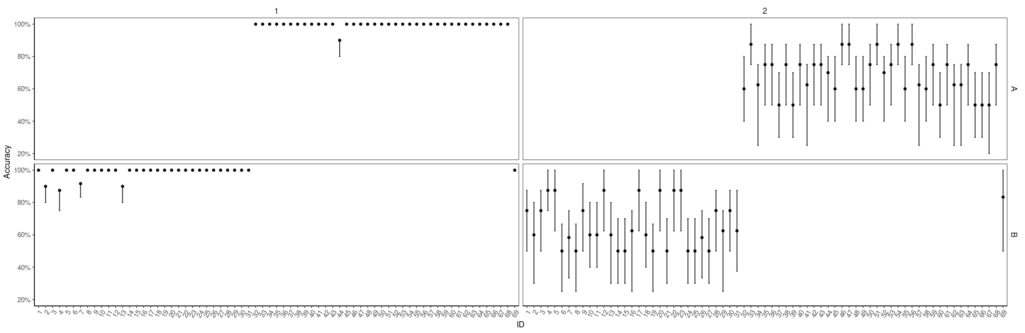
Look at accuracy
Data %>%
        add_predicted_draws(empty_Stan_Mod,
                            value = "Pred",
                            re_formula = NULL) %>%
        ungroup() %>%
        mutate(Correct = ifelse(Response == Pred, 1, 0)) %>%
        group_by(ID, Group, Type, .draw) %>%
        summarize(Accuracy = sum(Correct)/n()) %>%
        ungroup() %>%
        group_by(ID, Group, Type) %>%

        point_interval(Accuracy,
                       .width = 0.89,
                       .point = median,
                       .interval = hdci,
                       .simple_names = TRUE,
                       na.rm = TRUE) %>%
        ungroup() %>%

        ggplot(aes(reorder_within(ID, -Accuracy, Group), Accuracy)) +
        facet_grid(Group ~ Type, scales = "free_x") +
        geom_point(position = position_dodge(width = 0.5)) +
        geom_errorbar(aes(
                ymin = .lower,
                ymax = .upper),
                width = 0.2,
                position = position_dodge(width = 0.5)) +
        scale_x_reordered("ID") +
        scale_y_continuous("Accuracy", labels = scales::percent_format(accuracy = 1)) +
        theme_bw() +
        theme_bw() +
        theme(
                axis.text.x = element_text(angle = 60, hjust = 1, size = 10),
                axis.text.y = element_text(size = 10),
                axis.title.x = element_text(size = 12),
                axis.title.y = element_text(size = 12),
                plot.title = element_text(hjust = 0.5),
                panel.border = element_rect(fill = NA, colour = "black"),
                panel.grid.major = element_blank(),
                panel.grid.minor = element_blank(),
                axis.line = element_line(colour = "black"),
                strip.text.x = element_text(size = 12),
                strip.text.y = element_text(size = 12),
                strip.background = element_blank(),
                legend.title = element_blank(),
                legend.text = element_text(size = 10),
                legend.position = c(0.95, 0.05),
                legend.key = element_rect(fill = "transparent"),
                legend.direction = "horizontal",
                legend.background = element_rect(fill = "transparent", size = 6)
        )
I’d like to use generated quantities rather than fitting an empty model and replacing the fit slot.