Plotting logistic regressions with brms

Hello!

I was wondering if anyone had any experience with plotting predictions of a multivariate binomial model with brms? I will only provide the code for one response variable below.

All I get is this warning message:

Warning message:
Computation failed in stat_eye()
Caused by error in bw.SJ():
! sample is too sparse to find TD


My_model <- brm(FutureReproduction~ Reproductive_success+ Age 
     + Precipitation+ Scaled_Leg_index 
     + Reproductive_success*Age
     + (1 | ID),
     family = bernoulli()) 

condition <-expand.grid("Age" = (c(3, 4, 5, 6, 7,8, 9, 10, 11)),
                        Year = 2011,
                        ID = 3,
                        Precipitation= 0,
                        Leg_index= 0,
                        Reproductive_success = c(0, 1))


Model_prediction <- condition %>% 
  add_predicted_rvars(My_model, allow_new_levels = TRUE, re_formula = NA, newdata = .) %>% 
  mutate(Reproductive_success = factor(ifelse(Reproductive_success == 1, "Yes", "No"), levels = c("No", "Yes"))) 


> Model_prediction 
# A tibble: 18 × 7
     Age  Year    ID       Precipitation      Leg_index  Reproductive_success  prediction[,"Jumpheight"]  [,"Sprintspeed"] [,"Future Reproduction"] [,"Survival"]
   <dbl> <dbl> <dbl>              <dbl>            <dbl> <fct>                        <rvar[,1]>    <rvar[,1]>          <rvar[,1]>      <rvar[,1]>
 1     3  2011     3                  0                0 No                          21.33 ± 5.9    2.41 ± 1.8        0.261 ± 0.44     0.97 ± 0.18
 2     4  2011     3                  0                0 No                          10.63 ± 6.0    1.57 ± 1.8        0.230 ± 0.42     0.97 ± 0.17
 3     5  2011     3                  0                0 No                           4.60 ± 5.9    1.03 ± 1.8        0.202 ± 0.40     0.97 ± 0.18
 4     6  2011     3                  0                0 No                           2.49 ± 5.9    0.74 ± 1.8        0.188 ± 0.39     0.96 ± 0.19
 5     7  2011     3                  0                0 No                           2.63 ± 5.9    0.67 ± 1.8        0.168 ± 0.37     0.96 ± 0.19
 6     8  2011     3                  0                0 No                           3.59 ± 5.9    0.64 ± 1.8        0.153 ± 0.36     0.95 ± 0.22
 7     9  2011     3                  0                0 No                           5.12 ± 5.9    0.66 ± 1.8        0.148 ± 0.36     0.93 ± 0.25
 8    10  2011     3                  0                0 No                           6.88 ± 6.0    0.69 ± 1.8        0.136 ± 0.34     0.90 ± 0.29
 9    11  2011     3                  0                0 No                           8.97 ± 6.4    0.79 ± 1.9        0.134 ± 0.34     0.85 ± 0.35
10     3  2011     3                  0                0 Yes                          9.54 ± 6.6   -0.66 ± 2.0        0.029 ± 0.17     0.91 ± 0.28
11     4  2011     3                  0                0 Yes                          5.97 ± 5.9   -0.41 ± 1.8        0.025 ± 0.16     0.93 ± 0.25
12     5  2011     3                  0                0 Yes                          2.89 ± 6.1   -0.71 ± 1.8        0.022 ± 0.15     0.94 ± 0.23
13     6  2011     3                  0                0 Yes                          0.46 ± 6.0   -1.37 ± 1.8        0.018 ± 0.13     0.95 ± 0.23
14     7  2011     3                  0                0 Yes                         -1.18 ± 6.0   -2.11 ± 1.8        0.016 ± 0.13     0.95 ± 0.23
15     8  2011     3                  0                0 Yes                         -2.21 ± 6.1   -2.56 ± 1.8        0.017 ± 0.13     0.94 ± 0.24
16     9  2011     3                  0                0 Yes                         -2.53 ± 6.1   -2.63 ± 1.8        0.018 ± 0.13     0.92 ± 0.27
17    10  2011     3                  0                0 Yes                         -2.30 ± 6.2   -2.54 ± 1.8        0.017 ± 0.13     0.89 ± 0.32
18    11  2011     3                  0                0 Yes                         -1.54 ± 6.4   -2.22 ± 1.9        0.019 ± 0.14     0.86 ± 0.35

#Plot

Model_prediction %>% 
  ggplot(aes(x = Reproductive_success , ydist = .prediction[,"Future Reproduction"]) )+
  stat_eye()

Warning message:
Computation failed in `stat_eye()`
Caused by error in `bw.SJ()`:
! sample is too sparse to find TD 

I used the exact same approach for my other figures with gaussian distribution (continuous response variables) and had no issues

The issue here is likely caused by using a kernel density estimator (via ggdist::stat_eye()) on a discrete variable. In previous versions of ggdist, the default bandwidth estimator used by ggdist can sometimes fail on discrete data. If you update to the latest version, this should be fixed — it will now fall back to another bandwidth estimator in these cases. However, it will also give you a warning (worth heeding) that your data is likely discrete and therefore better suited to a histogram.

To get a histogram, you could replace stat_eye() with something like stat_eye(density = "histogram") or stat_histinterval(). If you want to enforce reasonable breaks for discrete data, maybe also pass something like breaks = breaks_fixed(width = 1), align = "center" to either function.

Alternatively, you can convert the underlying rvar column to a discrete rvar using as_rvar_integer() or as_rvar_factor(). If you attempt to visualize a discrete rvar with stat_eye() it will recognize that it is discrete and use a histogram with a bin width of 1 automatically.

I updated the packages and R, and it seemed to work a bit better, but the distributions are being wrapped to the top of the figure where the CrIs drop below 0, which led me to realize that I am using add_predicted_rvars incorrectly.

I believe having my response variable as a factor (Bernoulli) is part of my problem. I am a more used to epred / conditional effects to get a predicted posterior distribution which works fine for scatter plot with error bars (see first section of code) but I wanted to try to represent my data with density distributions to try and see the shape of the posterir distribution using add_predicted_rvars.

I realize that the add_predicted_rvars from the tidybayes package gives me a very different output (see second chunk of code and df).

I get very similar results between epred/ conditional_effects and add_predicted_rvars when I am using my a continuous response variable (see final chunk of code and plots)

Section 1

condition <-expand.grid(“Age” = c(3, 4, 5, 6, 7,8, 9, 10, 11),
Year = 2016,
ID = 495,
Scaled_Veg_per_roo = 0,
Scaled_Leg_index = 0)

Cde_weaning_shortterm = conditional_effects(Multivariate_model_ST,
resp=“WeaningstageFY”,
effect=“Weaning_stage”,
conditions = condition,
re_formula = NULL)

Weaning_RS_cde_shortterm = Cde_weaning_shortterm[[“WeaningstageFY.WeaningstageFY_Weaning_stage”]]

Weaning_RS_cde_shortterm %>%
ggplot(aes(x = Weaning_stage, y = estimate__))+
geom_errorbar(aes(ymin = lower__, ymax = upper__), size = 0.5, width = 0.5) +
geom_point(aes(fill = Age), shape = 21, size = 3) +
facet_wrap2(~ Age, scale = “free_x”) +
ylab(“Probability of future weaning”) +
xlab(“Young weaned”)

Weaning_RS_cde_shortterm %>%

  • filter(Age <6) %>% 
    
  • select(Age, Year, ID, Weaning_stage, estimate__, lower__, upper__)
    
    Age Year ID Weaning_stage estimate__ lower__ upper__
    1 3 2016 495 0 0.4693004 0.045165959 0.9482615
    2 3 2016 495 1 0.1256426 0.005269647 0.7211858
    3 4 2016 495 0 0.4523427 0.043885030 0.9413389
    4 4 2016 495 1 0.1198121 0.005488750 0.6904277
    5 5 2016 495 0 0.4364735 0.041315794 0.9364617
    6 5 2016 495 1 0.1168256 0.005585093 0.6740038

Section 2:

condition <-expand.grid(“Age” = (c(3, 4, 5, 6, 7,8, 9, 10, 11)),
Year = 2016,
ID = 495,
Scaled_Veg_per_roo = 0,
Scaled_Leg_index = 0,
Weaning_stage = c(0, 1))

RS_prediction_ST_cond ← condition %>%
add_predicted_rvars(Multivariate_model_ST, allow_new_levels = TRUE, re_formula = NA, newdata = .) %>%
mutate(Weaning_stage = factor(ifelse(Weaning_stage == 1, “Yes”, “No”), levels = c(“No”, “Yes”))) %>%
filter(Age<6)

RS_prediction_ST_cond

A tibble: 6 × 5

Age  Year    ID Weaning_stage .prediction[,"WeaningstageFY"]

<rvar[,1]>
1 3 2016 495 No 0.242 ± 0.43
2 4 2016 495 No 0.223 ± 0.42
3 5 2016 495 No 0.210 ± 0.41
4 3 2016 495 Yes 0.057 ± 0.23
5 4 2016 495 Yes 0.057 ± 0.23
6 5 2016 495 Yes 0.050 ± 0.22

RS_prediction_ST_cond %>%
ggplot() +
facet_wrap2(~ Age, scale = “free_x”) +
stat_halfeye(aes(ydist = .prediction[,“WeaningstageFY”], x = Weaning_stage,
fill = factor(Age), scale = 0.6),
position = position_dodge(width = 2)) +
labs(color = “Age”, fill = “Age”) +
ylab(“Predicted mass change (kg)”) +
xlab(“Young weaned”)

Section 3
#conditional_effects
condition <-expand.grid(“Age” = c(3, 4, 5, 6, 7,8, 9, 10, 11),
Year = 2023,
ID = 852,
Scaled_Veg_per_roo = 0,
Scaled_Leg_index = 0)

Weaning_mass_cde_short_term = conditional_effects(Multivariate_model_ST,
resp=“Massdiff”,
effect=“Weaning_stage”,
conditions = condition,
re_formula = NULL)

Weaning_mass_cde_short_term = Weaning_mass_cde_short_term[[“Massdiff.Massdiff_Weaning_stage”]] %>%
filter(Age < 6)

#add_r_vars
condition <-expand.grid(“Age” = (c(3, 4, 5, 6, 7,8, 9, 10, 11)),
Year = 2023,
ID = 852,
Scaled_Veg_per_roo = 0,
Scaled_Leg_index = 0,
Weaning_stage = c(0, 1))

Mass_prediction_ST_cond ← condition %>%
add_predicted_rvars(Multivariate_model_ST, allow_new_levels = TRUE, re_formula = NA, newdata = .) %>%
mutate(Weaning_stage = factor(ifelse(Weaning_stage == 1, “Yes”, “No”), levels = c(“No”, “Yes”))) %>%
filter(Age < 6)

#Df comparison
Weaning_mass_cde_short_term %>%

  • select(Age, Year, ID, Weaning_stage, estimate__, lower__, upper__)
    
    Age Year ID Weaning_stage estimate__ lower__ upper__
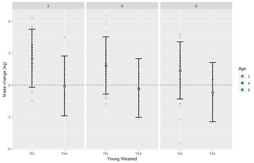
    1 3 2023 852 0 2.4671761 -0.2244421 5.218591
    2 3 2023 852 1 -0.1215248 -2.9110667 2.688034
    3 4 2023 852 0 1.7901435 -0.8587531 4.514089
    4 4 2023 852 1 -0.3471903 -3.0730995 2.455349
    5 5 2023 852 0 1.3258978 -1.3296359 4.030633
    6 5 2023 852 1 -0.7388673 -3.4639275 2.081341

Mass_prediction_ST_cond %>%

  • select(Age, Year, Weaning_stage, .prediction)
    

A tibble: 6 × 4

Age  Year Weaning_stage .prediction[,"Massdiff"] 

<rvar[,1]>
1 3 2023 No 2.46 ± 1.7
2 4 2023 No 1.80 ± 1.7
3 5 2023 No 1.32 ± 1.7
4 3 2023 Yes -0.13 ± 1.7
5 4 2023 Yes -0.37 ± 1.7
6 5 2023 Yes -0.74 ± 1.7

Scatteplot with error bars:

Halfeye plot:

add_epred_rvars(), posterior_epred(), and add_epred_draws() give you draws from the posterior distribution of the conditional mean. i.e. they quantify the uncertainty in the mean.

add_predicted_rvars(), posterior_predict(), and add_predicted_draws() give you draws from the posterior predictive distribution. i.e. they quantify uncertainty in new observations.

On a continuous distribution, these will tend to look similar (except that the uncertainty for the posterior predictive will be wider). On a discrete distribution, these won’t look similar, because the first one will give you (in the case of Bernoulli) the uncertainty in the probability of getting a 1 (a continuous value), and the second one will give you a discrete predictive distribution containing only 0s and 1s. More on this under Details here.