I have a least squares inference problem, and wanted to replace my Stan program with WLS. However, for some data, I get very different results, which I find very puzzling (see also here or here).
I am providing a specific example, with 29 data points, and the results of least squares and Stan. I simplified the problem to homoscadastic errors (yerr=1, i.e., OLS). In blue is a plot of the data:
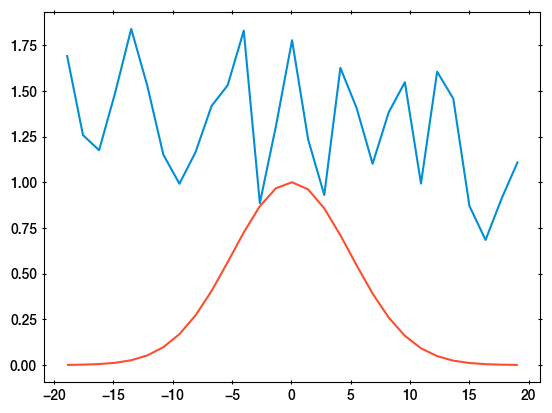
I fit with three components: 1) a constant, 2) a linear component, 3) a fixed shape (red curve). The normalisations are free parameters called y0, k, norm. They receive flat, unconstrained priors.
Below is my code, data and analysis:
import numpy as np
import cmdstanpy
import matplotlib.pyplot as plt
import corner
from statsmodels.regression.linear_model import WLS

# data:

data = {'N': 29, 'x0': 5895.6,
	'weight': np.array([7.8281132e-04, 2.0987201e-03, 5.2415314e-03, 1.2138436e-02,
       2.6183469e-02, 5.2412681e-02, 9.7503543e-02, 1.6878714e-01,
       2.7118218e-01, 4.0531352e-01, 5.6230277e-01, 7.2535461e-01,
       8.6879617e-01, 9.6697074e-01, 9.9991941e-01, 9.6047860e-01,
       8.5685223e-01, 7.1017146e-01, 5.4648513e-01, 3.9075232e-01,
       2.5953308e-01, 1.5991287e-01, 9.1608725e-02, 4.8663702e-02,
       2.4034550e-02, 1.1002056e-02, 4.6862061e-03, 1.8525344e-03,
       6.7856628e-04]),
       'x': np.array([5876.689 , 5878.041 , 5879.3965, 5880.7485, 5882.1045, 5883.458 ,
       5884.8115, 5886.1685, 5887.5225, 5888.8804, 5890.235 , 5891.5933,
       5892.948 , 5894.304 , 5895.6636, 5897.02  , 5898.3794, 5899.737 ,
       5901.0967, 5902.4546, 5903.8125, 5905.174 , 5906.532 , 5907.894 ,
       5909.2534, 5910.616 , 5911.9756, 5913.336 , 5914.699 ]),
      'y': np.array([1.6952891 , 1.2575909 , 1.1748848 , 1.488376  , 1.8385803 ,
       1.528486  , 1.1511977 , 0.9915795 , 1.1635164 , 1.4170816 ,
       1.5301417 , 1.8289143 , 0.8856548 , 1.3066483 , 1.7767009 ,
       1.2338594 , 0.93022835, 1.625354  , 1.4074879 , 1.1009187 ,
       1.3825897 , 1.546863  , 0.99267375, 1.6045758 , 1.4572536 ,
       0.8702313 , 0.68421644, 0.911552  , 1.1132364 ]),
       'yerr': np.array([1., 1., 1., 1., 1., 1., 1., 1., 1., 1., 1., 1., 1., 1., 1., 1., 1.,
       1., 1., 1., 1., 1., 1., 1., 1., 1., 1., 1., 1.])}
data['dx'] = data['x'] - data['x0']

# plot the data
plt.plot(data['dx'], data['y'])
plt.plot(data['dx'], data['weight'])
plt.savefig('wls-data.pdf')
plt.close()


# run WLS
# prepare WLS matrix
A = np.column_stack((np.ones(data['N']), data['dx'], data['weight']))
wls_results = WLS(data['y'], A, data['yerr']**-2).fit()
# wls_results = OLS(data['y'], A).fit()   # this gives the same results
params = wls_results.params
cov_matrix = wls_results.cov_params()
y0_fit, k_fit, norm_fit = params
y0_err, k_err, norm_err = np.sqrt(np.diag(cov_matrix))

# run Stan
# write the Stan code to a file
stan_code = """
data {
  int N;            // number of data points
  vector[N] dx;     // x data points
  vector[N] y;      // y data points
  vector[N] yerr;   // y uncertainty
  vector[N] weight; // weight describing feature shape
}
parameters {
  real y0;     // continuum normalisation
  real k;      // continuum slope
  real norm;   // feature strength
}
model {
  // assume Gaussian measurement errors
  y ~ normal(y0 + k * dx + norm * weight, yerr);
}
"""
model_name = 'wls'
filename = 'wls.stan'
with open(filename, 'w') as fout:
	fout.write(stan_code)

sm = cmdstanpy.CmdStanModel(stan_file=filename, model_name=model_name)
fit = sm.sample(data=data, iter_sampling=100000, iter_warmup=4000, chains=4, show_console=False, show_progress=True)
print(fit.summary())
print(fit.diagnose())
norm = fit.stan_variable('norm')
y0 = fit.stan_variable('y0')


# plot results:
corner.corner(
	np.transpose([y0, fit.stan_variable('k'), norm]), labels=['y0', 'k', 'norm'],
	plot_datapoints=False, plot_density=False, levels=np.exp(-np.arange(5)))
corner.corner(
	np.random.multivariate_normal(params, cov_matrix, size=len(norm)), labels=['y0', 'k', 'norm'],
	fig=plt.gcf(), color='b', plot_datapoints=False, plot_density=False, levels=np.exp(-np.arange(5)))
plt.savefig('wls_corner.pdf')

# compare means and errors of the two techniques:
print(' same norm?', norm_fit, norm.mean(), 'err:', norm_err, norm.std())
print(' same y0?', y0_fit, y0.mean(), 'err:', y0_err, y0.std())
The Stan diagnostics are all ok, and Rhat is 1.
I get the same means (first two numbers), but much larger uncertainties with Stan:
 same norm? 0.11509463050765173 0.11374671140722921 err: 0.15857910773382997 0.5286261376859842
 same y0? 1.2708374766432424 1.2714545692049999 err: 0.07524091396160146 0.25075389547048704
Here is a pairs/corner plot comparing the results from Stan (black) to the least squares covariance (blue):

Why do the results not coincide in this setting?