New to Stan - trying to estimate individual-level data using Bayesian inference

[jcohen]

I am brand new to Bayesian inference, Stan and Rstan. I am attempting to infer individual-level worm burdens based on individual-level egg outputs, initially just with very simple dummy data. I have generated dummy data:

#generate dummy data for worm counts, based on a negative binomial distribution
worms <- rnbinom(1000, size = 0.5, mu = 20)

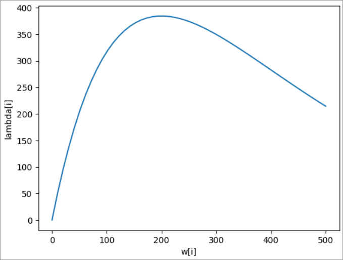
#density dependence of fecundity in worms
lambda <- ifelse(worms > 0, 5.2*worms*exp((worms - 1)*-0.005), 0)

#now use worm data to generate egg counts per individual
eggs <- rpois(length(worms), lambda)

I then set up a simple stan model:

// data block
data {
  int<lower = 0> N;
  array[N] int<lower = 0> egg_count; // egg count data
  real<lower = 0> fec; // worm fecundity
  real dd; // density dependence term
}

// parameter block
parameters {
  array[N] real<lower = 0> worms; // estimate worm number
}

// model block
model {
  // no priors
  // likelihood function
  for (i in 1:N) {
    egg_count[i] ~ poisson(fec*worms[i]*exp((worms[i] - 1)*dd)); // egg count is poisson distributed based on worms * fecundity * density dependence
  }
}

I then run the model using RStan:

#prepare dataset to pass to stan
worm_data <- list(N = length(eggs),
                  egg_count = eggs,
                  fec = 5.2,
                  dd = -0.005)

#run model
wb.model <- stan(
  file = "X.stan",
  data = worm_data,
  iter = 30000,
  chains = 3,
  verbose = FALSE
)

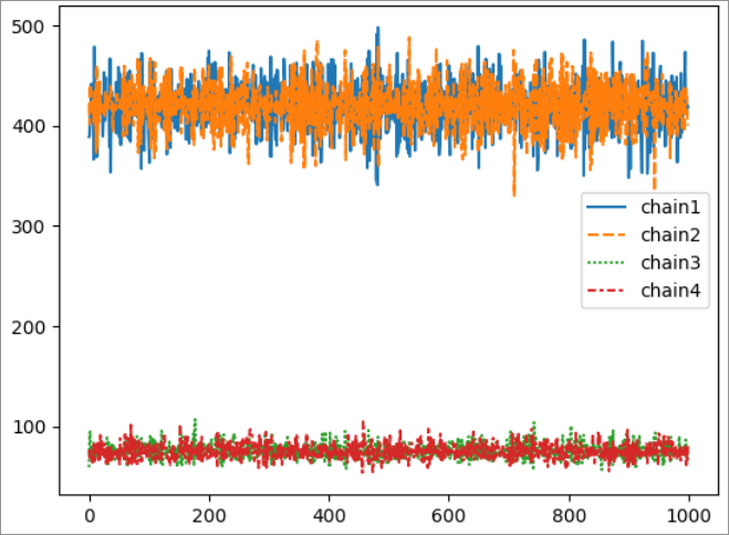
Weirdly, the model is able to infer worm burdens well at low egg count values, but does not converge at higher egg count values. I have tried increasing the iterations on the model, but it still does not converge.

What am I doing wrong?

Thanks in advance for the help.

[amas0]

Hi @jcohen and welcome to the Stan community!

Interesting issue – I used your code and was able to recreate the non-convergence, so let’s dig in. The first thing to note is that you don’t include any priors on this model – generally speaking that is something you should avoid doing. Even very weak containment priors tend to help quite a bit when it comes to efficient sampling. We’ll get back to this!

When I ran your code, I looked at the results and pulled the parameter that had the highest R-hat value. This is the traceplot for 4 chains:

We see an obvious case where two of the chains have localized around a parameter value of ~75 and the other two are around ~420 or so. This can signify that there’s an identifiability issue with your model where two different parameter values give equally good fits to the data.

To explore this further, I want to focus on the expression you provided:

\lambda_i = 5.2 w_i e^{-0.005 (w_i - 1)}

Let’s plot this as a function of w_i:

So what we see here are two distinct regions where a given value of \lambda_i can correspond to more than one value of w_i. In particular, we noted that in traceplot we had two modes at ~75 and ~420, computing the corresponding of \lambda_i, we get:

\lambda_i(75) \approx 269 \qquad \lambda_i(420) \approx 269

So our two modes correspond to identical inferences for w_i. This is almost definitely the source of your convergence issues. This can be solved with an appropriate prior on w_i. To decide what to set, you would need to think about what region of w_i makes sense, based on your expertise, to constrain the values of w_i.

I re-ran the model with the prior:

worms ~ normal(0, 30);

and the convergence warnings disappeared. I don’t know if that prior makes sense, but it gives you an idea of the approach you can take to address these issues.

[jcohen]

Hi @amas0 and thanks for your response. This makes sense to me, and I’ll be more careful about choosing density dependent terms in future.

Out of curiosity, if this density dependent term were the observed curve in the biological system, what would you do (apart from setting potentially biologically unrealistic priors) to try and get convergence?

[amas0]

Good question.

So let’s take your particular example, where the expected observed egg counts are determined by this curve that is dependent on the worm count. If your goal is to use the observed egg counts to infer the worm counts, then this means that the egg counts alone do not provide enough information to distinguish between the modes in this model.

I’m not a biologist, but I would guess the motivation here is that at low worm counts, increasing the number of worms proportionally increases the number of observed eggs. At some point, however, competition or other constraints mean that the ability to produce eggs decreases. So by observing egg counts, we get the low-mode (where the behavior is primarily driven by increasing worm count) and the high-mode (where behavior is primarily driven by the constraints). In this model, we do not have enough information to distinguish between them.

As mentioned, a stronger prior is one mechanism you can use to distinguish which mode the inferred worm counts should belong to, but absent that, you would need some additional structural information in the model. If there are any other variables that can be observed that would correlate with worm counts (but not exhibit the same identifiability issues), then that can be included to help resolve the issue.

It’s worth noting that these convergence issues only really apply to your inferences of the worm counts, the rate parameter lambda should be inferred properly by this model.

So the next steps I would ask are:

1. What is the specific inference goal of the model? Is it to accurately identify worm counts?
2. What additional information could I potentially add into my model to expand it and resolve the identifiability issue? Are stronger priors appropriate? Are there additional experimental data that can be collected?

Note, this is an excellent example of why building a model and working with dummy data can be so valuable. If you are doing this before you conduct your experiments/collect your data, then you know that you may need to change up your experimental design to account for this.