Update: I have since been able to make this (kind of) work in #interfaces:brms using the awesome custom family capabilities.
Here’s the custom family call. Based on this discussion I tried using the “categorical” special option , but couldn’t get it to work because I kept getting messages about the number of categories, so did it the manual way. If anyone has any thoughts on this, please share!
library(brms)
library(readr)
library(dplyr)
library(rstan)
library(bayesplot)

# create custom family for zero inflated ordinal
# define two parameters (mu and eta), one for the zero inflation (mu)
# and one for the regular ordinal part (eta)
# also have to define the (threshold) intercept variable (c_int)
zi_ordinal <- custom_family(
  "zi_ordinal", dpars = c("mu", "eta"),
  links = c("identity"), lb = c(NA, NA),
  type = c("int"), vars = c("c_int")
)


# define stan functions
# we define the lpmf and the random number generator
stan_funs <- stanvar(block = "functions", scode = "
  real zi_ordinal_lpmf(int k, real mu, real eta, vector c_int) {
      if (k == 0) // assume non-response coded as 0
        return bernoulli_logit_lpmf(1| mu); // predict non-response with probability p
      else // otherwise use ordered logistic with prob 1-p
        return bernoulli_logit_lpmf(0| mu) + ordered_logistic_lpmf(k | eta, c_int);
  }
  int zi_ordinal_rng(real mu, real eta, vector c_int) {
    if (bernoulli_rng(inv_logit(mu)) == 1)
      return 0;
    else
      return ordered_logistic_rng(eta, c_int);
  }
")

# this feels sort of hacky, but to define the ordered c_int variable i had to
# add this to the parameters block, as well as the number of categories (n_thresh)
ordered_var <- stanvar(scode = "ordered[n_thresh] c_int;", block = "parameters")
ncat_var <- stanvar(x = 3, name = "n_thresh", scode = "int n_thresh;")
stanvars <- ordered_var + ncat_var + stan_funs
This seems to work fine. The parameters recovered are the same as the Stan model (shown above).
# read in data
data <- read_csv("https://raw.githubusercontent.com/octmedina/zi-ordinal/main/merkel_data.csv")

# fit the model. it works!
fit_zi_ord <- brm(
  bf(confid_merkel ~ 1 + party + income + edu + race,
     eta ~ 0 + party + income + edu + race),
  data = data,
  family = zi_ordinal, stanvars = stanvars,
  chains = 2,
  cores = 2
)

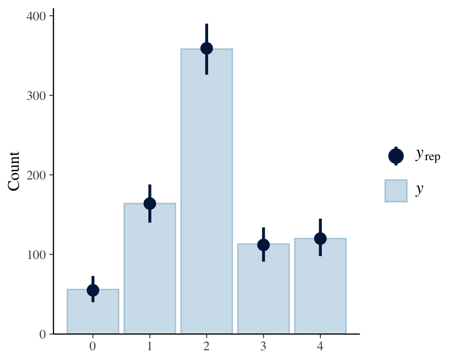
But here’s something that I’ve been struggling with. The posterior predictive checks look similar, except the intervals are way wider! I don’t really know why, since it seems that the parameters are similar, and the predicted values are also similar for every observation. Could it be the way I’m generating the samples? I used the categorical distribution to generate them.
# Create posterior predict function for post-processing
posterior_predict_zi_ordinal <- function(i, prep, ...) {
  c_all <- rstan::extract(fit_zi_ord$fit, pars = "c_int") # extract intercepts
  c_int <- as.matrix(c_all$c_int[,1:3]) # convert to matrix

  mu <- brms::get_dpar(prep, "mu", i = i) # get mu (zero/non-response inflation)
  eta <- brms::get_dpar(prep, "eta", i = i) # get eta (regular ordinal logistic)

  p_zi <- plogis(mu) # inverse-logit
  thresholds <- ncol(c_int) # get number of thresholds

  # create the probabilities for all the categories
  p_total <- cbind(p_zi, (1-p_zi)*(1-plogis(eta-c_int[,1])))
  for (val in 2:thresholds) {
    p_total <- cbind(p_total, (1-p_zi)*(plogis(eta-c_int[,val-1])-plogis(eta-c_int[,val])))
  }
  p_total <- cbind(p_total, (1-p_zi)*(plogis(eta-c_int[,thresholds])))

  # generate samples (subtract 1 bc first category is 0)
  y_rep <- extraDistr::rcat(n=dim(p_total)[1], prob = p_total)-1
  y_rep <- as.matrix(y_rep)
  y_rep
}

# Generate samples (seems to work)
brms_yrep <- posterior_predict(fit_zi_ord)
Here are the two bayesplot outputs, for comparison. The Rstan model is available in the message above, and the full reprex is here.