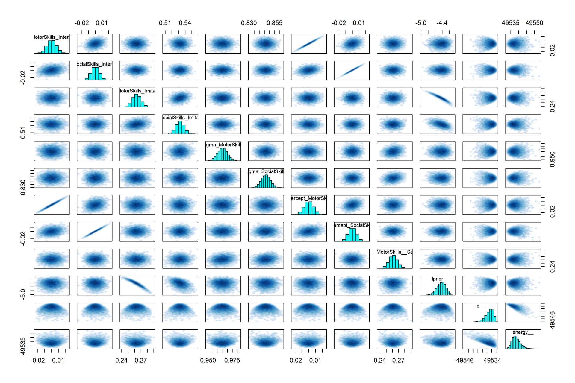
I’ve run a relatively simplistic multivariate outcome with “Imitation” as a common cause of “Motor.Skills” and “Social.Skills” in brms. I had no issues with convergence, no other warnings, and the parameters replicate the frequentist model (in lavaan). Looking at the pairs plot, there is a nearly perfect correlation between lprior and b_MotorSkills_Imitation; my understanding is that this is driven by the narrower prior for b_MotorSkills_Imitation; the lprior reflects. I re-ran the model with each beta parameter’s having equal variance (.1) and now the b_SocialSkills_Imitation parameter correlates strongly with lprior.
My questions are two-fold:
- Why are there duplicated intercept terms (2 for each model) in the pairs plot? This seems inefficient, given their extremely strong correlation.
- Is a correlation between lprior and a slope parameter necessarily problematic? I’ve looked at the priorsense GitHub, and am trying to get it working on my models.
ME_priors <- c(prior(normal(.22, .05), class="b", coef = "Imitation", resp = "MotorSkills"),
               prior(normal(.46, .12), class="b", coef = "Imitation", resp = "SocialSkills"))

mot.pred <- bf(Motor.Skills ~ Imitation)
soc.pred <- bf(Social.Skills ~ Imitation)

ME_sem_fit_rescor_brms <- brm(
  mot.pred + soc.pred + set_rescor(TRUE),
  data = data2,
  prior = ME_priors,
  warmup = 1000, iter = 3500,
  cores = 4, chains = 4,
  file = "./brms_models/ME_rescor_10000.rds"
)

data2 <- structure(c(-1.08, 0.18, 0.18, 1.44, 1.44, -1.08, -1.08, 1.44,
            0.18, 0.18, -1.08, -1.08, -1.08, -1.08, -1.08, -1.08, 1.44, -1.08,
            1.44, 0.18, 0.18, 0.18, -1.08, -1.08, 0.18, 0.18, -1.08, -1.08,
            1.44, -1.08, -1.08, -1.08, -1.08, -1.08, -1.08, 1.44, -1.08,
            0.18, 1.44, 1.44, 1.44, -1.08, -1.08, -1.08, -1.08, 0.18, 0.18,
            -1.08, -1.08, -1.08, -1.08, 0.18, -1.08, 0.18, -1.08, 0.18, 0.18,
            0.18, 0.18, 0.18, -1.08, -1.08, -1.08, 1.44, 1.44, -1.08, 0.18,
            0.18, -1.08, 0.18, 0.18, -1.08, 0.18, 0.18, 0.18, 0.18, 0.18,
            0.18, 1.44, 0.18, -1.08, -1.08, -1.08, -1.08, 1.44, 1.44, 1.44,
            0.18, -1.08, -1.08, 0.18, 0.18, 0.18, -1.08, -1.08, 0.18, -1.08,
            -1.08, 1.44, -1.08, -0.88, -0.53, -0.31, -0.21, 1.52, -1.07,
            -1.21, 0.21, 0.14, -0.03, 1.11, -0.16, -0.29, -1.08, 1.3, -1.56,
            1.99, 0.83, -0.25, 0.13, -0.95, -1.62, -0.52, -0.85, 0.73, 0.96,
            -0.37, -0.91, -1.46, 0.44, -0.74, -0.75, -1.54, 0.27, -0.82,
            0.46, 0.68, -0.32, -0.01, 1.11, 0.4, -1.74, 0.26, -1.74, -1.25,
            -0.67, -0.35, -1.04, 0.13, -1.33, 1.28, -0.07, -0.89, 0.48, 0.5,
            -0.65, -1.74, -0.61, 0.73, -1.03, -0.35, 0.2, 1.22, 1.98, 1.06,
            -1.44, -0.56, -1.74, -1.74, -0.74, -0.59, 0.39, 2.18, 1.19, 0.76,
            0.39, -1.42, -0.14, 0.97, 0.26, -1.07, 0.81, -0.91, -0.69, 0.73,
            0.67, 0.39, 0.26, -0.68, 0.95, 0.35, -1.25, -0.19, -0.97, -0.5,
            -0.19, -1.03, -0.91, -0.05, -0.86, -0.96, -0.04, -1.17, 0.78,
            2.12, -0.92, 0.55, 1.61, 0.07, 0.78, 0.75, -0.13, -0.13, -1.69,
            -0.95, -1.51, 0.58, 0.04, 1.84, 0.34, -2.12, -1.34, -0.78, -0.39,
            -0.91, 0.74, 0.38, -0.76, 0.38, -0.52, -0.65, 0.42, -0.28, -0.86,
            -0.74, 1.56, -0.62, -0.46, 0.64, -0.14, -0.22, -0.52, -0.9, -1.64,
            -0.52, -0.23, 0.93, -1.03, 0.47, -1.74, -1.83, -1.72, -0.68,
            -0.56, -0.61, -0.05, 0.65, 0.09, 0.76, -0.77, -0.58, -1.38, 0.31,
            0.79, 1.44, -0.8, 1.64, 0.49, -1.64, -0.39, -0.76, -0.33, 0.89,
            -1.23, 0.36, 1.84, -1.44, 0.38, -0.44, 1.3, 0.24, 0.53, -0.04,
            -0.81, 2.12, 2.12, 0.76, 0.88, -1.21, -1.02, -0.34, 0.18, -0.94,
            -1.69, -1.02, 0.14, -1.23, -0.81, -0.93, -0.65), dim = c(100L,
                                                                     3L))

 Family: MV(gaussian, gaussian)
  Links: mu = identity; sigma = identity
         mu = identity; sigma = identity
Formula: Motor.Skills ~ Imitation
         Social.Skills ~ Imitation
   Data: data2 (Number of observations: 19053)
  Draws: 4 chains, each with iter = 3500; warmup = 1000; thin = 1;
         total post-warmup draws = 10000

Regression Coefficients:
                       Estimate Est.Error l-95% CI u-95% CI Rhat Bulk_ESS Tail_ESS
MotorSkills_Intercept      0.00      0.01    -0.01     0.01 1.00    13776     7568
SocialSkills_Intercept    -0.00      0.01    -0.01     0.01 1.00    13952     8046
MotorSkills_Imitation      0.26      0.01     0.25     0.28 1.00    14713     8124
SocialSkills_Imitation     0.53      0.01     0.52     0.54 1.00    13807     7507

Further Distributional Parameters:
                   Estimate Est.Error l-95% CI u-95% CI Rhat Bulk_ESS Tail_ESS
sigma_MotorSkills      0.96      0.00     0.96     0.97 1.00    15741     7794
sigma_SocialSkills     0.85      0.00     0.84     0.85 1.00    16427     8456

Residual Correlations:
                                 Estimate Est.Error l-95% CI u-95% CI Rhat Bulk_ESS Tail_ESS
rescor(MotorSkills,SocialSkills)     0.26      0.01     0.25     0.27 1.00    13799     8123

Draws were sampled using sampling(NUTS). For each parameter, Bulk_ESS
and Tail_ESS are effective sample size measures, and Rhat is the potential
scale reduction factor on split chains (at convergence, Rhat = 1).
First plot is from code above
Second plot is from code above with altered priors, such that var is .1 for each

- Operating System: Windows 10 Enterprise
- brms Version: 2.22.0