Hello,
I am working on a joint model in which the two equations are related. The equations are the following:
\hat{trait_i} = \alpha_{grand} + \alpha sp_{sp_i} + \alpha study_{study_i}
\alpha sp \sim N(0, \sigma_{sp})
\alpha study \sim N(0, \sigma_{study})
trait_i \sim N(\hat{trait}_i, \sigma_{trait})
\hat{pheno}_i = \alpha pheno_{sp_i} + \beta force_{sp_i} * Forcing_{i} + \beta photo_{sp_i} * Photo_{i} + \beta chill_{sp_i} * Chill_{i}
\beta force_{sp} = \alpha force_{sp} + \beta trait.force * \alpha sp_{sp}
\beta chill_{sp} = \alpha chill_{sp} + \beta trait.chill * \alpha sp_{sp}
\beta photo_{sp} = \alpha photo_{sp} + \beta trait.photo * \alpha sp_{sp}
\alpha pheno \sim N(\mu_{pheno}, \sigma_{pheno})
\alpha force \sim N(\mu_{force}, \sigma_{force})
\alpha chill \sim N(\mu_{chill}, \sigma_{chill})
\alpha photo \sim N(\mu_{photo}, \sigma_{photo})
pheno_{i} \sim N(\hat{pheno_i}, \sigma_{pheno})
The associated Stan code is:
data {
    //MODEL 1 ------------------------------------------------
    int < lower = 1 > N; // Sample size for trait data
    int < lower = 1 > n_study; // number of random effect levels (study)
    int < lower = 1, upper = n_study > study[N]; // id of random effect (study)
    vector[N] yTraiti; // trait data

    //both models --------------------------------------------------------
    int < lower = 1 > n_spec; // number of random effect levels (species)
    int < lower = 1, upper = n_spec > species[N]; // id of random effect (species)

    //MODEL 2 ------------------------------------------------
    int < lower = 1 > Nph;
    vector[Nph] yPhenoi;// phenology
    vector[Nph] forcei; // predictor forcing
    vector[Nph] photoi; // predictor photoperiod
    vector[Nph] chilli; // predictor chilling

    int < lower = 1, upper = n_spec > species2[Nph]; // id of random effect (species)
}

parameters{
    //MODEL 1 ------------------------------------------------

    real <lower =0> sigmaTrait_y; // overall variation accross trait observations
    real mu_grand; // grand mean for trait values
    real <lower = 0> sigma_sp; // variation of intercepts amoung species
    real muSp[n_spec]; //the trait effect of each species without study
    real <lower = 0> sigma_study; // variation of intercept amoung studies
    real muStudy[n_study]; // mean of the alpha value for studies

    //MODEL 2 -----------------------------------------------------
    real alphaForceSp[n_spec]; //the distribution of species forcing values
    real muForceSp; // the mean of the effect of forcing
    real <lower = 0> sigmaForceSp; //variation around the mean of the effect of forcing

    real alphaChillSp[n_spec];
    real muChillSp;
    real <lower = 0> sigmaChillSp;

    real alphaPhotoSp[n_spec];
    real muPhotoSp;
    real <lower = 0> sigmaPhotoSp;

    real alphaPhenoSp[n_spec];
    real muPhenoSp; //
    real <lower = 0> sigmaPhenoSp;

    real betaTraitxForce;
    real betaTraitxChill;
    real betaTraitxPhoto;

    real <lower =0> sigmapheno_y;
}

transformed parameters{
    //MODEL 1 ----------------------------------------
    //Individual mean for species and study
    real ymu[N]; // the trait value

    //MODEL 2------------------------------------------------
    real betaForceSp[n_spec];     //species level beta forcing
    real betaPhotoSp[n_spec];     //species level beta photoperiod
    real betaChillSp[n_spec];     //species level beta chilling

    //MODEL 1
    //Individual mean calculation
    for (i in 1:N){
        ymu[i] = mu_grand + muSp[species[i]] + muStudy[study[i]];  //
    }

    //MODEL 2----------------------------------------
    for (isp in 1:n_spec){
    betaForceSp[isp] = alphaForceSp[isp] + betaTraitxForce * ( muSp[isp]);
    }

    for (isp in 1:n_spec){
    betaPhotoSp[isp] = alphaPhotoSp[isp] + betaTraitxPhoto* ( muSp[isp]);
    }

    for (isp in 1:n_spec){
    betaChillSp[isp] = alphaChillSp[isp] + betaTraitxChill* (muSp[isp]);
    }
}
model{
    //MODEL 1 ---------------------------------------------
sigmaTrait_y ~ normal(15,1); //
    sigma_sp ~ normal(10,1); //
    mu_grand ~ normal(10, 1); //
    muSp ~ normal(0, sigma_sp); //

    sigma_study ~ normal(5,1); //
    muStudy ~ normal(0, sigma_study);//

    for (i in 1:N){
        yTraiti[i] ~ normal(ymu[i], sigmaTrait_y);
    }

    //MODEL 2 -----------------------------------------------
    //priors - level 1
    sigmapheno_y ~ normal(5, 3); //

    //priors level 2
    sigmaForceSp ~ normal(5, 0.1); //
    muForceSp ~ normal(-1, 0.5);//
    alphaForceSp ~ normal(muForceSp, sigmaForceSp);  //

    sigmaChillSp ~ normal(5, 0.5); //
    muChillSp ~ normal(-2, 0.5);//
    alphaChillSp ~ normal(muChillSp, sigmaChillSp);  //

    sigmaPhotoSp ~ normal(5, 0.5); //
    muPhotoSp ~ normal(-2, 0.5);//
    alphaPhotoSp ~ normal(muPhotoSp, sigmaPhotoSp);  //

    sigmaPhenoSp ~ normal(10, 1); //
    muPhenoSp ~ normal(150, 10);  //
    alphaPhenoSp ~ normal(muPhenoSp, sigmaPhenoSp);//

    betaTraitxForce ~ normal(0, 1); //
    betaTraitxPhoto ~ normal(0, 1); //
    betaTraitxChill ~ normal(0, 1); //

        for (i in 1:Nph){
    yPhenoi[i] ~ normal( alphaPhenoSp[species2[i]] + betaForceSp[species2[i]] * forcei[i] + betaPhotoSp[species2[i]] * photoi[i] + betaChillSp[species2[i]] * chilli[i], sigmapheno_y);
        }
}
The aim of this model is to test the relationship between plant functional traits (height, leaf mass per area, seed size, etc) and environmental cues (spring forcing temperatures, winter chilling temperatures, and photoperiod) effects on plant budburst dates. Our model includes latent variables that allow us to quantify the trait’s effect on phenology for each cue separately (\beta traitxForce). We also have partial pooling across species and study as a random effect.
I have worked up the code using test data, and the model runs. The R code used to generate the test data is :
##########################################################################
#Trait model
##########################################################################
Nrep <- 10 # rep per trait
Nstudy <- 25 # number of studies w/ traits
Nspp <- 40 # number of species with traits

# Test trait data:
Ntrt <- Nspp * Nstudy * Nrep # total number of traits observations
Ntrt

#make a dataframe for trait1
trt.dat <- data.frame(matrix(NA, Ntrt, 1))
names(trt.dat) <- c("rep")
trt.dat$rep <- c(1:Nrep)
trt.dat$study <- rep(c(1:Nstudy), each = Nspp)
trt.dat$species <- rep(1:Nspp, Nstudy)

# Generating the species trait data
mu.grand <- 10 # the grand mean of the trait model
sigma.species <- 10 # Variaiton across species

mu.trtsp <- rnorm(Nspp, 0, sigma.species)
trt.dat$mu.trtsp <- rep(mu.trtsp, Nstudy) #adding trait data for ea. sp

#now generating the effects of study (differences in observers, methods, etc)
sigma.study <- 5
mu.study <- rnorm(Nstudy, 0, sigma.study) #intercept for each study
trt.dat$mu.study <- rep(mu.study, each = Nspp)

# general trait variance
trt.var <- 15 #sigmaTrait_y in the stan code
trt.dat$trt.er <- rnorm(Ntrt, 0, trt.var)

trt.dat$yTraiti <- mu.grand + trt.dat$mu.trtsp + trt.dat$mu.study + trt.dat$trt.er

##########################################################################
#Phenology model
##########################################################################

Nspp <- 40 # number of species
nphen <- 15 # reps per phenological event
Nph <- Nspp * nphen
Nph

# Test phenology data:
pheno.dat <- data.frame(matrix(NA, Nph, 2))
names(pheno.dat) <- c("rep","species")
pheno.dat$rep <- c(1:Nph)
pheno.dat$species <- rep(c(1:Nspp), each = nphen)

# Generating data for the environmental cues: winter chilling (chill), spring forcing (force), and photoperiod (photo)

# Phenological values across the different species
mu.pheno.sp <- 150
sigma.pheno.sp <- 10
alpha.pheno.sp <- rnorm(Nspp, mu.pheno.sp, sigma.pheno.sp)
pheno.dat$alpha.pheno.sp <- rep(alpha.pheno.sp, each = nphen)

mu.force.sp <- -1
sigma.force.sp <- 5
alpha.force.sp <- rnorm(Nspp, mu.force.sp, sigma.force.sp)
pheno.dat$alpha.force.sp <- rep(alpha.force.sp, each = nphen)

mu.chill.sp <- -2
sigma.chill.sp <- 5
alpha.chill.sp <- rnorm(Nspp, mu.chill.sp, sigma.chill.sp)
pheno.dat$alpha.chill.sp <- rep(alpha.chill.sp, each = nphen)

mu.photo.sp <- -2 # negative bc warmer means earlier
sigma.photo.sp <- 5
alpha.photo.sp <- rnorm(Nspp, mu.photo.sp, sigma.photo.sp)
pheno.dat$alpha.photo.sp <- rep(alpha.photo.sp, each = nphen)

betaTraitxforce <- 0 #interaction between trait and phenology
betaTraitxchill <- 0 #interaction between trait and phenology
betaTraitxphoto <- 0 #interaction between trait and phenology

beta.force.temp <- alpha.force.sp + mu.trtsp * betaTraitxforce
beta.force.sp <- rep(beta.force.temp,)
pheno.dat$beta.force.sp <- rep(beta.force.sp, each = nphen)

beta.chill.temp <- alpha.chill.sp + mu.trtsp * betaTraitxchill
beta.chill.sp <- rep(beta.chill.temp,)
pheno.dat$beta.chill.sp <- rep(beta.chill.sp, each = nphen)

beta.photo.temp <- alpha.photo.sp + mu.trtsp * betaTraitxphoto
beta.photo.sp <- rep(beta.photo.temp,)
pheno.dat$beta.photo.sp <- rep(beta.photo.sp, each = nphen)

#Generate the cue values
mu.force <- 5
sigma.force <- 1
force.i <- rnorm(Nph, mu.force, sigma.force)  # predictor forcing, forcei in stan
pheno.dat$force.i <- force.i

mu.chill <- 5
sigma.chill <- 1
chill.i <- rnorm(Nph, mu.chill, sigma.chill)  # predictor chilling, chilli in stan
pheno.dat$chill.i <- chill.i

mu.photo <- 5
sigma.photo <- 1
photo.i <- rnorm(Nph, mu.photo, sigma.photo)  # predictor photoperiod, photoi in stan
pheno.dat$photo.i <- photo.i

#general phenology variance
sigma.gen <- 5
gen.var <- rnorm(Nph, 0, sigma.gen)
pheno.dat$gen.er <- gen.var

#the full model simulating data
pheno.dat$doy.i <- pheno.dat$alpha.pheno.sp + pheno.dat$beta.force.sp * pheno.dat$force.i + pheno.dat$beta.chill.sp * pheno.dat$chill.i + pheno.dat$beta.photo.sp * pheno.dat$photo.i + pheno.dat$gen.er
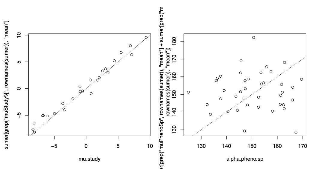
But we found the addition of the third climate cue to produce low n_eff values for our muSp[n] and muStudy[n] estimates (as low as 280). Of greater concern was the poor chain mixing we observed for these parameters.

The estimated values for muStudy (shown on the left figures y-axis) do correlate well with the test data, but the estimates for muSpecies are quite poor (right figure).
My issues are that I have not been able to correct the poorly mixing chains and low n_eff. It is unclear to me what about the model with three cues is causing this or whether there is something that I am simply missing.
Any suggestions or insights into how to improve this model would be greatly appreciated. Thanks!