My own data rather more complicated than anything I’ve presented here but are in the slightly ambiguous domain I’d say. I wanted to gain confidence in the simple cases before building up to the full set of structures informed by domain expertise. I’ll actually be dealing with N latent periodic timeseries, decently separated in frequency but each with a gradual time-varying frequency and amplitude, that in turn influence M observed timeseries. The influence of the n^{th} latent series on the m^{th} observed series includes a weight W_{nm} as well as a phase-offset \Delta_{nm}, and finally the m^{th} observed series has it’s own magnitude of measurement noise \sigma_m; all of these quantities being time-invariant. SNRs are such that after looking at lots of data I’ve been able to derive pretty high confidence in this structure, but not so high that I’d trust non-Bayesian methods (MLE, or simple FFT-and-peak-finding) for reliable inference. And ultimately this entire structure is to capture known noise structure, with yet another quasi-periodic latent signal of interest buried well beneath SNR-wise.
I think @martinmodrak’s solution would be a great case study (or even short research paper), especially given that you’ve searched around and it’s a relatively open problem. I’m really interested in the cases where this will not work too (put another way what assumptions must hold for this to work). I’d also like to put it in a function and add to my helpful stan functions repo.
Yeah, I was definitely thinking that @martinmodrak should publish this approach. If it helps, here’s some code to generate and fit across a wide range on inputs:test.r (2.2 KB)
I think I’ve got something for the “less than slightly ambiguous” domain.

Some explanation will follow.
I admit I scanned a lot of the earlier comments, so apologies if I misunderstood something. My main point was that it can be useful to think in terms of the frequency domain rather than just the time domain. (And beyond that, working with wavelets can be useful, though perhaps not relevant here.)
Regarding the Dirac delta function, it’s slightly more complex (ha!) than I stated in my reply, but not much — have a look at a table of Fourier transform pairs.
As a suggestion for where to look outside astrophysics, take a look at medical physics and medical imaging. For example, look at reconstruction of MRI images from undersampled data, particularly the post-Nyquist era work. This is obviously a different and more complex problem than discussed here, but it might provide some useful insights.
Hm, okay, you’ll have to wait some more for the explanation of the above figure. I was hoping that the same procedure that could take care of multimodality for ODEs could do so for this problem, but it turns out it only works reliably when the other modes are truly unreasonable.
Anyhow, Martin’s approach worked so well that I decided to adapt and accidentally extend it.
There are some (remaining) issues:
- Sometimes the frequency is negative. Not sure how big an issue this is.
- I’m not a fan of the arbitrariness of
x_fixed. I think settingx_fixedto the bounds is reasonable. Then every additionalkcorresponds to one more period over all of the data. - The runtime depends quite strongly on
max_k. I believe for unambiguous data a lot of time could be saved by incrementally fitting the data and restrictingkto somemin_k,…,max_kwhich are selected based on the minima/maxima of the previous fits.
This is a slightly simplified/modified/extended version of @martinmodrak’s model:
functions{
	// https://en.wikipedia.org/wiki/Rotation_matrix
	matrix rotation_matrix(real phi){
		return to_matrix({
				{cos(phi), -sin(phi)},
				{sin(phi), cos(phi)}
		});
	}
}
data{
	int n ;
	vector[n] x;
	vector[n] y;
	int max_k;
}
transformed data{
	real dx = x[n] - x[1];
	vector[n] rel_x = (x - x[1]) / dx;
}
parameters{
	vector[2] z_left;
	vector[2] z_right;
	real<lower=0> noise;
}
transformed parameters{
	vector[max_k+1] candidate_frequencies;
	vector[max_k+1] log_likelihoods;
	real amp_left = sqrt(dot_self(z_left));
	real phase_left = atan2(z_left[1],z_left[2]);
	real amp_right = sqrt(dot_self(z_right));
	vector[2] rel_z = rotation_matrix(-phase_left) * z_right;
	real dphase = atan2(rel_z[1],rel_z[2]);
	for(k in 1:max_k+1){
		real omega = (k-1)*2*pi()+dphase;
		vector[n] yk = (
				amp_left + (amp_right - amp_left) * rel_x
			) .* sin(omega*rel_x+phase_left);
		log_likelihoods[k] = normal_lpdf(y | yk, noise);
		candidate_frequencies[k] = omega/(2*pi()*dx);
	}
}
model{
	target += -log(amp_left);
	target += -log(amp_right);
	amp_left ~ weibull(2,1);
	amp_right ~ weibull(2,1);
	noise ~ weibull(2,1);
	target += log_sum_exp(log_likelihoods);
}
generated quantities{
	real frequency = candidate_frequencies[categorical_logit_rng(log_likelihoods)];
}
And this is how the models perform for artifical data with max_k=n/2:
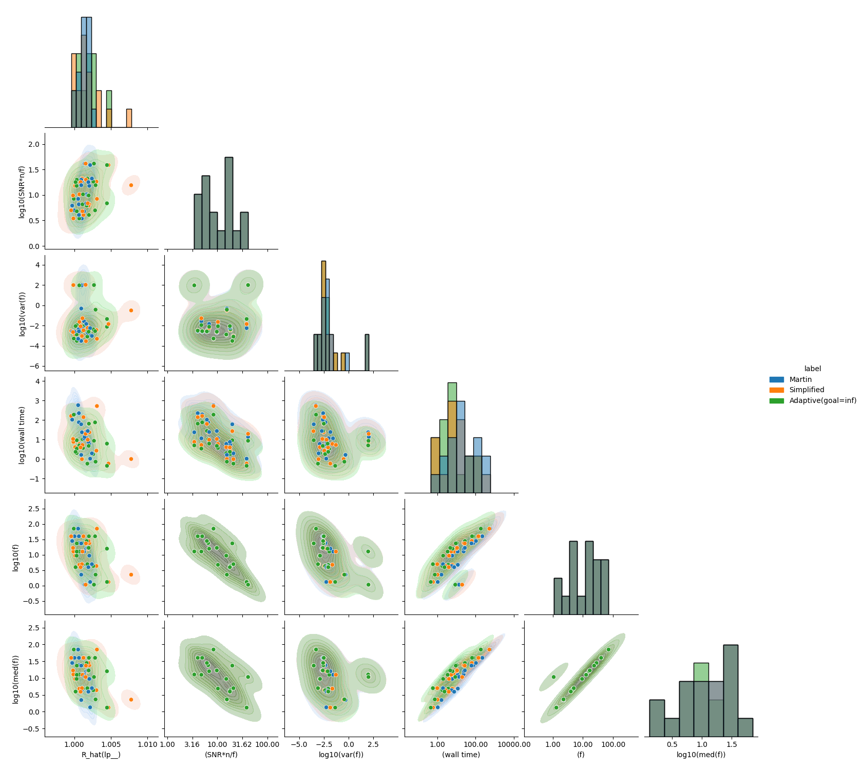
Disclaimer: Green corresponds to the simplified model using a simple incremental warmup.
Generally for periodic data, the sampling rate could be seen as a rough guide to the data-collector’s bounds on the prior for the frequency of the signals of interest, so we’d generally collect data such that there is at least 1 period of the function of interest in the data set, and at a rate such that we get at least 4 data points for the fastest frequency. So (assuming a fixed sample rate) would it make sense to set min_k=1 (or maybe .5?) and max_k = (x[n]-x[1])/((x[2]-x[1])*4)? Or am I not understanding the parameterization quite right?
Hm, I think the parametrization is (in this aspect) the same as @martinmodrak’s. For his and for my parametrization, k=0 and k=1 may correspond to f<=1. (It is slightly weird).
Edit with more info:
Yes, on X=(0,1) with n+1 equidistant measurement points, this would correspond to f \in (1,n/4) which is roughly equivalent to min_k=0 and max_k=n/4 if xfixed = {0,1}. Accounting for the possibility of underresolved frequencies, we may set e.g. max_k=n/2.
On the other hand, if xfixed is e.g. xfixed={0,.5}, then (I think) f \in (1,n/4) is roughly equivalent to max_k=n/8 (with min_k=0 implicit). I’m not 100% sure, it’s slightly confusing:
Anyhow, with min_k=0 and max_k=n/2 (picked to frustrate the non-adaptive version), n >= 4*f and f \in (1,100), an adaptive-version quite dramatically outperforms the non-adaptive version for “large” n and f and datasets that are informative enough to effectively bound the frequency:

I think I’ve got a reliable and (relatively fast) method for linear superpositions of waves that should work for an “arbitrary” number of waves.
Example:

More to come.
I currently don’t have the time/resources to start another project. If anybody feels like this is useful and worthy of their time, I’d be glad to see it developed further. I can also definitely consult a bit or clarify some stuff if that helps, but that’s about all.
I think that to have z well informed by the data, it is helpful that x_fixed are surrounded by data on both sides. If the sampling is roughly uniform, then a better default would IMHO be putting x_fixed at 1st and 3rd quarter of the observed range, so increasing k by one means up to 2 more periods over the whole range. So still quite interpretable but hopefully better behaved.
I think putting boudns on k would be important for efficiency, but I think the approach mentioned is a bit risky if the data actually don’t inform k that well - as seen in the last example of the original post one could have a relatively wide region of k values with low posterior probability before an additional mode. So in cases where one suspects multiple relevant modes, this heuristic might be problematic.
If on the other hand one is sure that the posterior should have just one well-defined mode I think it is actually pretty safe to just init all the chains within the mode (as in the Planetary motion example in the Bayesian Workflow preprint ). If the mode turns out to not be se well defined, you will get divergences/Rhat issues so the cases when setting inits leads to invalid inferences without warnings would IMHO be quite rare (it would only be an issue if there are multiple modes with non-negligibla posterior mass well separated from any other such modes by regions of negligible posterior mass).
@mike-lawrence standard approach in astrophysics for looking for the frequency is the Lomb-Scargle periodogram. This handles unevenly spaced data too.
@mike-lawrence you should look at Numerical Recipies in C section 13.4
This problem has been well studied. The additional likelihood modes are unavoidable based on the fact that you have a window of finite size. They will decrease in amplitude as the window size increases.
Also, any sampling difficulties you have here are due to the choice of sampler and the multi-modal behaviour. NUTS uses the local gradient, which is efficient for unimodal problems, but can get trapped if the scaling is wrong.
If you used Gibbs sampling based on slice sampling you wouldn’t have any issues with multi-modality.
Good call. I came directly to Stan in my path to Bayes, so likely have my sense of what’s possible constrained by what Stan is good at (which, as you say, seems to be unimodal/continuous-gradient scenarios).
I looked at frequency-domain stuff a bit a while ago and at first thought I’d discovered the cause of the multimodality as deriving from an implicit rectangluar window function (i.e. implied by not using any windowing of the input signal), but abandoned that idea after realizing it doesn’t account for the asymmetry.
Doesn’t it? I may well have misunderstood the problem, because to me this does look like the solution.
As you say, we are considering infinite sinusoids but we are observing only a finite section – a “rectangular window” – from them. The fourier transform of the infinite sinusoid is an impulse, but multiplying the sinusoid by a rectangular window smears this out into a main lobe of finite width centred on the sinusoid frequency, and also adds side lobes that create the multimodality.
In practical terms, the sidelobes arise because if the sinusoid has 10 cycles in the window (as in this example) then a sinusoid with 9 or 11 cycles can fit the ends of the data well while being little correlated in the middle. Consequently it is guaranteed to fit better overall than a sinusoid with 9.5 or 10.5 cycles that must be little correlated overall. More generally, any sinusoid of any frequency that has the correct phases at both edges of a rectangular window will fit better than a sinusoid that fits in half a cycle more or less because the latter cannot fit at both ends. This creates infinite modes.
However, all but one of these modes are just artefacts created by the finite window, and if the window had no edges there would be no edge effects. These artefacts are typically unwanted and methods to deal with them are very well known, the key being to use a window that is smoother in the time domain than is the rectangular window, with the smooth function chosen in such a way that the frequency domain sidelobes are suppressed. The classic Hann window w = (1-cos(2 * pi * t))/2 for t in the range 0 to 1 is an elegant and well-behaved example.
However, like most windows Hann focusses on reducing rather than eliminating sidelobes, and the only window I know that is claimed to entirely eliminate them is the Hann–Poisson window. This multiplies a Hann window with a Poisson one, w = exp(-2 * a * abs(t-0.5)) * (1-cos(2 * pi * t))/2 for some parameter a>=2.
This has the unusual property that a sinusoid observed through this window will have a unimodal likelihood function. Provided we are prepared to formulate priors that involve a Hann-Poisson windowed sinusoid rather than a rectangularly windowed one, I think we should be able to sample from the posterior without any particular difficulty…? I would also expect this approach to work with the other examples of problematic periodic series, such as planetary motion and the asymmetric sinusoid.
Robert Macrae
Ah, thanks @rmac for chiming in. I definitely appreciate that windowing is a feasible solution to the batched-inference scenario that has been presented up to this point in the thread, but ultimately I’ll be looking to deploy to realtime contexts with sequential updating (I know stan doesn’t do that at present, but @s.maskell has work in the pipeline to enable this, and tensorflow Probability already has sequential MC options).
Also, even in the batched case, I’ll be looking to eventually model a time-varying rate, which windowing will impair.
More generally, I really feel that windowing must surely be unnecessary even in the batched-and-constant-rate scenario. I’m a cognitive scientist, so I know it’s dangerous to assume the brain is ever fully rational or computationally optimal, but I can’t help shake the intuition that the fact that a human observer can clearly come to a unimodal state when looking at periodic data suggests that there is math to achieve the same. But maybe that’s an artifact of my log-scale depictions of the probability distributions; certainly in many scenarios the brain has built-in reassignment of small probabilities to zero, possibly aiding the sense of conscious experience of unimodal belief…
Is that right? I think it is only the prior that has to be specified in terms of windowed series, you can still use every observation and can still update online.
I was once involved in a project modeling quasi-periodic signals with alternating frequency, amplitude and shifts Dynamic Retrospective Filtering of Physiological Noise in BOLD fMRI: DRIFTER. But the inference there goes beoynd Stan.
I have tried using a Hann-Poisson window to solve the problem… and it works when little noise is present but not as well as I hoped. I have put live code on Colab courtesy Mitzi Morris, CmdStanPy and Google in case any of it is useful but TLDR: probably not the way to go.
The code in Mike-Lawrence’ post of 22 Apr 2021 contains two sources of multimodality: sidelobes due to the rectangular window, and aliased frequencies above the Nyquist limit. These can be addressed by the Hann-Poisson window and limiting frequencies to lie under the Nyquist frequency. The revised code now expresses a prior about the frequency of a continuous wavelet with an H-P profile and its centre in the middle of the observed data, rather than about the frequency of a sine wave observed through a rectangular window. Clearly these are two different objects so inferences are slightly indirect; for example I adjust the profile of the noise to be higher towards the ends of the sample where by construction the wavelet cannot explain the data.
This version does seem to work a little better than using a sine prior when only low levels of noise are present in the data, and it consistently samples from a small span around the correct frequency. Unfortunately, even with well-behaved Gaussian white noise problems start to appear as the noise power approaches the signal power, with erratic and unconvincing sampling from the other peaks that are becoming prominent parts of the spectrum. I assume similar problem would arise if more than one sine were present, so I doubt there are many real situations in which this approach would be competitive with classical estimators.
Perhaps a frequency domain solution is more promising? This attempt tried to sample a simple, 2-parameter object (the sine or wavelet) from a space that has a complex geometry. However, Stan isn’t bothered by high dimensions and it should be possible to instead sample a whole spectrum from a space that has a simpler geometry…?