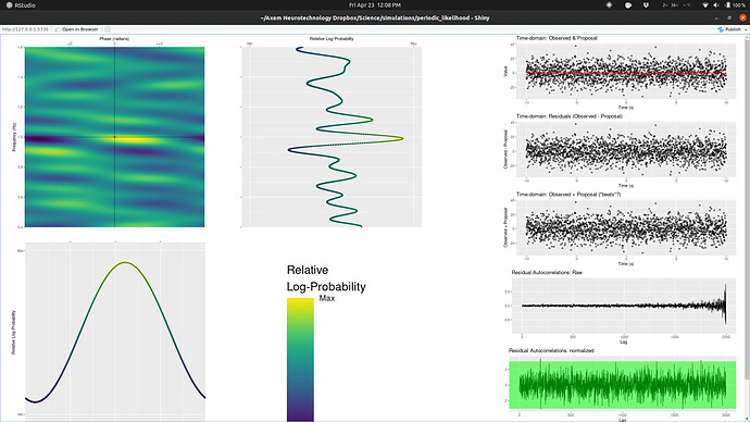
Ideas for modelling a periodic timeseries

So given a simple sinusoid-measured-noisily, one would think a straightforward model like this would be sufficient:

data{
	int n ;
	vector[n] y ; 
	vector[n] x ;
}
transformed data{
	vector[n] y_scaled = (y-mean(y))/sd(y) ;
}
parameters{
	real<lower=0> noise ;
	real<lower=0> frequency ; 
	vector[2] phamp ; // phase & amplitude (but a transform thereof)
}
transformed parameters{
	real amp = sqrt(dot_self(phamp));
	real phase = atan2(phamp[1],phamp[2]);
	vector[n] f = amp * sin(x*frequency - phase) ;
}
model{
	noise ~ weibull(2,1) ; //peaked at ~.8, zero-at-zero, ~2% mass >2
	amp ~ weibull(2,1) ; //ditto
	target += log(amp) ; // jacobian for setting a prior on amp given it's derivation from phamp
	// phase has an implied uniform prior
	frequency ~ ... ; // prior on frequency should account for the range and spacing of x
	y_scaled ~ normal(f,noise) ;
}

But it turns out that the likelihood topography (code to generate/explore here)
of even this simple model is massively multimodal:


in the frequency dimension in a confoundingly complex manner (i.e. itā€™s not just harmonics), causing typical multimodal sampling issues (different chains finding different modes).

Iā€™ve cast a wide net in trying to find solutions to this, including bugging a bunch of astrophysics folks who I imagined must encounter this issue a ton, but so far as I can tell no one has developed any robust solutions to this (the astro folks seem to have contented themselves with simply doing a maximum-likelihoood search in a very constrained frequency range).

While itā€™s straightforward to reframe things as a Gaussian Process with a periodic kernel, this can be very compute-intensive (something Iā€™d like to avoid as ultimately Iā€™ll be looking to do inference in a realtime context), so Iā€™ve been trying to come up with alternative solutions. I recently started learning about Hidden Markov Models, insipring a couple possible applications of HMMs to this periodic signals problem. My first thought was to model the derivative of the periodic signal as positive or negative, and that works to a degree, but felt pretty kludgey.

Then I realized that the derivative part is unnecessary (well, for sinusoids at least), leading me to think about the general structure whereby a periodic signal is modelled as an HMM with K states reflecting K ordered means with a transition matrix such that each state has a non-zero probability of transitioning to only itā€™s neighbors:

data{
	int n ;
	vector[n] y ; // assumed to be scaled with zero mean
	int<lower=3> k ; //must be odd
}
transformed data{
	int j = (k-1)/2 ;  // num states on either side of the halfway state
}
parameters{
	simplex[k] p0 ; // initial state probabilities
	simplex[3] tp_arr[k-2] ; // transition probability for all but the most extreme
	simplex[2] tp_ext[2] ; //transition probabilities for the extreme-most states
	positive_ordered[j] m_pos ; // state means (should these maybe be simply equidistant?)
	// positive_ordered[j] m_neg ; // for a sinusoid, can assume neg means same spacing as pos means
	real<lower=0> noise ; //measurement noise
}
transformed parameters {
	vector[k] m ;
	m[j+1] = 0.0 ; // halfway state has 0 mean
	for(i_j in 1:j){
		// m[(j+1)-i_j] = -m_neg[i_j] ;
		m[(j+1)-i_j] = -m_pos[i_j] ;
		m[(j+1)+i_j] = m_pos[i_j] ;
	}
	matrix[k, k] tp_mat = rep_matrix(0,k,k) ;
	for(i_k in 2:(k-1)){
		tp_mat[i_k,(i_k-1):(i_k+1)] = tp_arr[i_k-1]' ;
	}
	tp_mat[1,1:2] = tp_ext[1]' ;
	tp_mat[k,(k-1):k] = tp_ext[2]' ;
	matrix[k, n] state_ll ;
	for(i_n in 1:n) {
		for(i_k in 1:k){
			state_ll[i_k,i_n] = normal_lpdf(y[i_n]|m[i_k],noise) ;
		}
	}
}
model{
	noise ~ std_normal() ;
	m_pos ~ std_normal() ;
	// m_neg ~ std_normal() ;
	target += hmm_marginal(state_ll, tp_mat, p0) ;
}
generated quantities{
	vector[n] fk ;
	vector[n] fm ;
	{
		matrix[k,n] p = hmm_hidden_state_prob(state_ll, tp_mat, p0) ;
		for(i_n in 1:n){
			real highest_p = 0 ;
			for(i_k in 1:k){
				if(p[i_k,i_n]>highest_p){
					highest_p = p[i_k,i_n] ;
					fk[i_n] = i_k ;
					fm[i_n] = m[i_k] ;
				}
			}
		}
	}
}

With this model, as K increases, we get more states that are closer together and thereby smoother and smoother realizations of data y. Iā€™m thinking then that maybe thereā€™s math that works out a representation for the limit of K=\infty, where I suspect the frequency of the true signal will determine the structure of the transition matrix, or whatever limit-level entity serves the role of the transition matrix.

But Iā€™m super math-untrained, so thought Iā€™d query the folks here on whether thatā€™s possible. Thoughts anyone?

(One thing Iā€™ll add as a post script: as expressed above, the sequential-K HMM only weakly implicates periodicity whereby each state should have an equal chance of proceeding to either of itā€™s neighbors. This ā€œfitsā€ periodic data where we pass through the state going both ways, but doesnā€™t fully reflect that the previous state determines the transition probabilities of the current state. But I guess thatā€™s the fundamental nature/point of HMMs? And if I want to convey a transition thatā€™s deterministic, Iā€™m back in the function world of the first model above? I still wonder if some additional useful constraint might be achieved by, in addition to the HMM on the raw signal, also doing an HMM on the derivative, which I think would imply/induce the kind of transition directionality Iā€™m thinking might be more periodic-accurate.)

5 Likes

I believe the states in an HMM are said to probabilistic follow a multinomial distribution. When the number of states, K \to \infty, it follows a continuous state process. If you assume that a normal distribution approximates this process then use a Kalman filter.

See page 9 https://arxiv.org/pdf/1811.11618.pdf. Also Durbin and Koopman but I donā€™t have the book handy right now.

Iā€™ll ping @helske @JuhoKokkala @jrnold @Charles_Driver who have implementations of Kalman filters in Stan and may be able to help.

3 Likes

Hey @mike-lawrence,

Neat to see how this has been coming along! I donā€™t have any useful answers to your questions, but do have one question/comment (possibly irrelevant or harebrained):

In the examples that youā€™re working with, the approximate period is trivial to infer by just eyeballing the data, which points the way towards doing what the astrophysicists apparently do (although you could do it with a Bayesian estimation approach by using a strong prior on the period). It seems like the more dangerous case is if the data are noisy enough that you cannot unambiguously infer the approximate period (to within, say, 25% or so, which is where the spurious modes start to become a potential issue). But have you confirmed that the severe multimodality actually persists in this regime? That is, if the data are noisy enough that the approximate period isnā€™t obvious, then does that also flatten out the modes and connect them sufficiently for robust HMC exploration?

Cheers
Jacob

Yes for the continuous form Iā€™ve an example here: ctsem Quick Start -- Sunspots Damped Linear Oscillator | Charles Driver
If youā€™ve got equally spaced observations and donā€™t care about a generative model then you can also use the discrete time form to skip some of the heavier computation. Donā€™t know if this helps but if you want to chat briefly on it sometime feel free to ping meā€¦

4 Likes

And those modes are unreasonable?

As others mentioned, a huge influence on what a solution would look like is whether the secondary modes can be safely assumed negligible (and you just need a way for them to not break sampling) or if they should actually (at least in some cases) appear in the model posteriorā€¦

If the secondary modes are negligible, then just figuring out good inits should let you get rid of them (as in the Planetary motion case study). If they are not, I think a possible approach for the latter case might be to split the frequency spectrum into bins that should contain at most a single mode each (those could be determined by some preprocessing or maybe known from theory). You would then marginalize out a discrete indexing variable over those bins (and have a copy of all of the curve parameters for each bin). Maybe even estimating an ordered vector of frequencies could work together with such marginalizationā€¦ But I am purely speculating here.

In general I think that stochastic differential equations are another continuous analog to HMMs, but those are AFAIK very hard to solve and Stan has no SDE capabilities built-in.

1 Like

Itā€™s not that difficult to automatically sample from the ā€œbestā€ mode, is it?

But how do we (automatically) decide whether the other modes are unimportant?

1 Like

Thanks all for responding!! Some replies below:

Ah, neat! Iā€™d just recently started trying to wrap my head around Kalman filters too, and this makes total sense as the limit representation. Thanks! Oh, and also for the paper; Iā€™d read this and this but still working on really groking things.

Ooh, good point. Iā€™d been exploring the topography in the low-noise case bc I wanted to really get at the core of why the pathology manifests even for really clean data. Unfortunately after exploring just now, it seems the multimodality gets worse with increased noise. The above is from an SNR=10, hereā€™s SNR=1 (frequency range zoomed in to reduce compute):

And hereā€™s SNR = .1:

Ah, so the linear-oscillator rabbit hole I took myself down months ago wasnā€™t crazy! I canā€™t remember why I abandoned that line, and am having trouble following your vignette, but I am at the moment mostly interested in the discrete time scenario so will definitely take you up on your offer to discuss fast solutions in that context!

Yes. They seem to be happening when the frequency is slightly off but aligns with the data very slightly. For example, hereā€™s the mode at the frequency just higher than the true frequency:

Yeah, one hack Iā€™ve done was run a quick FFT to determine inits, but felt that was both inelegant and likely to be fragile in higher noise regimes.

I definitely got lost in trying to follow this idea šŸ˜³

3 Likes

Mike, this fits really well. Constraining the regression variate to -1 and 1 and putting an arcsine prior on it. I made it really close to your simulation but it also fits well albeit with higher sdā€™s if you remove z. Not sure if this will work for your more general case but maybe a start.

functions {
    real arcsine_lpdf ( vector x ) {
    int N = num_elements(x);
    return -N * log(pi()) - 
           sum( 0.5 * ( log1p( x ) + log1m( x ) ) );
  } 
}
data {
  int<lower=0> N;
  vector[N] y;
}
parameters {
  vector<lower=-1, upper=1>[N] x;
  vector<lower=-1, upper=1>[N] z;
  real<lower=0> sigma;
}
model {
  sigma ~ exponential(1);
  x ~ arcsine();
  z ~ arcsine();
 
  y ~ normal(sin(x + sin(z)), sigma);
}
generated quantities {
  vector[N] f;
  
  for (n in 1:N) 
    f[n] = normal_rng(sin(x[n] + sin(z[n])), sigma);
  
}

fit = mod$sample(
  data = list(
    N = nrow(dat)
    , y = dat$y),
  max_treedepth = 10,
  adapt_delta = 0.8,
  iter_warmup = 400,
  iter_sampling = 400,
  parallel_chains = 4,
  seed = 12341
)

fit$cmdstan_diagnose()

where that showed no bmfi warnings like I had with just fitting x or even constraining x within -1, 1 but no arcsine prior.

Processing csv files: /tmp/Rtmpr4aIZS/sine-202104231520-1-7c05c6.csv, /tmp/Rtmpr4aIZS/sine-202104231520-2-7c05c6.csv, /tmp/Rtmpr4aIZS/sine-202104231520-3-7c05c6.csv, /tmp/Rtmpr4aIZS/sine-202104231520-4-7c05c6.csv

Checking sampler transitions treedepth.
Treedepth satisfactory for all transitions.

Checking sampler transitions for divergences.
No divergent transitions found.

Checking E-BFMI - sampler transitions HMC potential energy.
E-BFMI satisfactory for all transitions.

Effective sample size satisfactory.

Split R-hat values satisfactory all parameters.

Processing complete, no problems detected.
4 Likes

Yowie! Thatā€™s wild!

I just messed around with my arcsine stuff with noise of 0.8 HMC worked fine. It did take over a minute to sample with 400 wu, 400 iters. The issue is that there are 2 * N parameters. But I think if Mike messes around with the regression he can get down to some K < N.

# generate data ----
set.seed(1)
dat = (
  tibble(
    time = seq(0,10,by=1/100)
    , f_true = asym_sine(time,hz=3,phase=0.3)
    , y = f_true + rnorm(length(time),0,.8)
    , y_std =( y - mean(y) ) / ( 2 * sd(y) )
  )
)

> fit = mod$sample(
+   data = list(
+     N = nrow(dat)
+     , y = dat$y),
+   max_treedepth = 10,
+   adapt_delta = 0.8,
+  refresh = 0,
+    iter_warmup = 400,
+   iter_sampling = 400,
+   parallel_chains = 4,
+   seed = 12341
+ )
Running MCMC with 4 parallel chains...

Chain 4 Informational Message: The current Metropolis proposal is about to be rejected because of the following issue:
Chain 4 Exception: normal_lpdf: Scale parameter is 0, but must be positive! (in '/tmp/Rtmpr4aIZS/model-790642ebef45d.stan', line 29, column 2 to column 37)
Chain 4 If this warning occurs sporadically, such as for highly constrained variable types like covariance matrices, then the sampler is fine,
Chain 4 but if this warning occurs often then your model may be either severely ill-conditioned or misspecified.
Chain 4 
Chain 2 finished in 62.1 seconds.
Chain 3 finished in 67.3 seconds.
Chain 1 finished in 70.0 seconds.
Chain 4 finished in 80.2 seconds.

All 4 chains finished successfully.
Mean chain execution time: 69.9 seconds.
Total execution time: 80.5 seconds.
> 
> fit$cmdstan_diagnose()
Processing csv files: /tmp/Rtmpr4aIZS/sine-202104231549-1-98e989.csv, /tmp/Rtmpr4aIZS/sine-202104231549-2-98e989.csv, /tmp/Rtmpr4aIZS/sine-202104231549-3-98e989.csv, /tmp/Rtmpr4aIZS/sine-202104231549-4-98e989.csv

Checking sampler transitions treedepth.
Treedepth satisfactory for all transitions.

Checking sampler transitions for divergences.
No divergent transitions found.

Checking E-BFMI - sampler transitions HMC potential energy.
E-BFMI satisfactory for all transitions.

Effective sample size satisfactory.

Split R-hat values satisfactory all parameters.

Processing complete, no problems detected.
2 Likes

In addition to what @mike-lawrence already mentioned, Iā€™ll add that (at least for clean nearly sinusoidal data that are evenly distributed across the domain), the spurious modes correspond to frequencies so that the number of full periods on the domain differs from the true value by either an integer or by an integer plus one half (IIRC the difference is full integers for periods that differ from the true period in one direction, and integers-plus-one-half for periods that differ in the other direction, but I forget which direction is which!).

I donā€™t understand why this is true mathematically, but that seems to be what happens. One consequence of this is that the distance separating the modes decreases as the number of periods on the domain increases.

Ah, right, I remember back when we discussed this on Slack you worked out that relation. Itā€™s some sort of Beat phenomenon, which you can see it in the residuals of the off-global-maximum mode plot above.

That is so clever! I never would have thought of getting the model to do inference on the covariate! Off to play with this!

@spinkney Why the -1:1 limits on x & z? Shouldnā€™t they be -pi:pi? Or are the limits arbitrary?

Oh, itā€™s bc of the arcsine prior, which is only defined for values between -1 and 1.

@spinkney So with your model, weā€™re doing inference on a latent vector thatā€™s given an arcsine prior that I donā€™t fully understand but seems to treat each element independently (i.e. the prior doesnā€™t impose any kind of smooth transitions between elements).

Playing with it, I get the same results as you post (once I standardize the y-range range to about -1:1 as your ystd, or add an amplitude parameter so that vector[n] f = amp * sin(x+sin(z)) ;) for the case of an asymmetric sinusoid generating function, high sample rate and moderate noise. Interestingly it success in that case seems to rely on the asymmertric structure, as if I switch to a sinusoid and even decrease the noise in the data generation, it has a lot of trouble (inc. divergences). It also definitely has trouble as noise increases or sample rate decreases.

How about a ā€œchallengeā€ prior?

I.e. a prior from which we can draw samples and do SBC?

@mike-lawrence this is great! Iā€™ve really wanted to use the inverse stereographic normal distribution! See https://projecteuclid.org/download/pdfview_1/euclid.ejs/1566353061

Try this
edit: needed a prior on mu.

functions {
   real isnorm_lpdf(vector x, real mu, real sigma) {
     // real log_constant = -0.5 * log(2 * pi());
     int N = num_elements(x);
     vector[N] cos1p = cos(x) + 1;
     real first = -sum(log(cos1p) + log(sigma));
     real second = -0.5 / square(sigma);
     real third = sum(second * square( ( sin(x) ./ cos1p ) -  mu ));
     
     return first + third;
   }
}
data {
  int<lower=0> N;
  vector[N] y;
  vector[N] time;
}

parameters {
  real mu;
  real<lower=0> sigma[2];
  vector<lower=-pi(), upper=pi()>[N] z;
}
model {
  mu ~ std_normal();
  sigma ~ exponential(1);
  z ~ isnorm(mu, sigma[1]);
  y ~ normal(sin(z), sigma[2]);
}
generated quantities {
  vector[N] f;
  
  for (n in 1:N) 
    f[n] = normal_rng(sin(z[n]), sigma[2]);
  
}

I just tested how regular HMC performs, higher SNRs seem to be more problematic. A slightly adapted warmup has no problems.

Hm, Iā€™m getting terrible fits across the board with it; have I messed something up in my alteration of the priors or naming somewhere?

functions {
	 real isnorm_lpdf(vector x, real mu, real sigma) {
		 // real log_constant = -0.5 * log(2 * pi());
		 int n = num_elements(x);
		 vector[n] cos1p = cos(x) + 1;
		 real first = -sum(log(cos1p) + log(sigma));
		 real second = -0.5 / square(sigma);
		 real third = sum(second * square( ( sin(x) ./ cos1p ) -  mu ));

		 return first + third;
	 }
}
data {
	int<lower=0> n;
	vector[n] y;
}
parameters {
	real<lower=0> noise ;
	real<lower=0> amp ;
	vector<lower=-pi(), upper=pi()>[n] z;
	real z_m;
	real<lower=0> z_s;
}
transformed parameters{
	vector[n] f = amp*sin(z);
}
model {
	noise ~ weibull(2,1) ;
	amp ~ weibull(2,1) ;
	z_m ~ std_normal() ;
	z_s ~ weibull(2,1) ;
	z ~ isnorm(z_m, z_s);
	y ~ normal(f, noise);
}
generated quantities {
	vector[n] yrep;
	for (i_n in 1:n){
		yrep[i_n] = normal_rng(f[i_n], noise);
	}
}