How to interpret MCMC model result

Hi everyone,

I’m new to bayesian inference, especially running MCMC for parameter inference. So, I have successfully run my model, but I do not think that I got the result as I expected (see the result below, I have 11 theta, and 1 sigma parameters, all of them do not have good n_eff and R_hat values).

            mean	se_mean	sd	 2.50%	  25%	 50%	75%	  97.50%	n_eff	Rhat
theta[1]    1.99    0.97   0.97   1.02   1.02   1.99   2.96   2.96      1  1.6e4
theta[2]     0.9    0.27   0.27   0.63   0.63    0.9   1.17   1.18      1 9874.4
theta[3]    10.0  8.9e-7 2.3e-5   10.0   10.0   10.0   10.0   10.0    675    1.0
theta[4]    3.08    1.63   1.63   1.44   1.44   3.08   4.71   4.71      1  1.4e4
theta[5]    2.22    1.45   1.45   0.76   0.76   2.22   3.67   3.67      1  1.7e4
theta[6]    0.14  4.6e-4 4.6e-4   0.14   0.14   0.14   0.14   0.14      1 118.71
theta[7]    0.52    0.19   0.19   0.33   0.33   0.52   0.71   0.71      1 7263.1
theta[8]    0.74    0.26   0.26   0.48   0.48   0.74    1.0    1.0      1 6272.7
theta[9]  3.0e-5  3.1e-5 1.4e-4 1.8e-6 2.8e-6 4.3e-6 8.3e-6 2.8e-4     20   1.07
theta[10]   1.09     0.9    0.9   0.19   0.19   1.09   1.99   1.99      1  2.3e4
theta[11]   0.43    0.24   0.24   0.19   0.19   0.43   0.67   0.67      1  1.7e4
sigma     288.66    0.27   0.61 287.67 288.14 288.64 289.22 289.65      5   2.23
lp__      -8.0e6   2.0e4  2.7e4 -8.0e6 -8.0e6 -8.0e6 -7.9e6 -7.9e6      2   1.59

Now, it seems the problem came from incorrect parameter initialization, but honestly I have no idea how I can determine these (I was just using uniform distribution with arbitrary ranges, as follows):

theta[1] ~ uniform(0, 1e1);
theta[2] ~ uniform(0, 1e1);
theta[3] ~ uniform(0, 1e1);
theta[4] ~ uniform(0, 1e2);
theta[5] ~ uniform(0, 1e2);
theta[6] ~ uniform(0, 1e-4);
theta[7] ~ uniform(0, 1e-1);
theta[8] ~ uniform(0, 1e0);
theta[9] ~ uniform(0, 1e5);
theta[10] ~ uniform(0, 1e2);
theta[11] ~ uniform(0, 4);
sigma ~ normal(0, 0.1);

I have tried tweaking the sampling parameters, such as iter, warmup, thin, and adapt_delta but none of these seem to work. I am just confused what kind of information that I can get out of this result that can guide me to improve the model. Can anyone tell me, typically, when improving a MCMC model what do guys look into? Because right now, I am just tweaking every possible number without any idea how that will hypothetically improve my model, and then I ended up spending multiple hours of try and error without any promising result. If anyone can share your rule of thumb in doing model parameter estimation with MCMC, that will be great too.

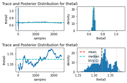
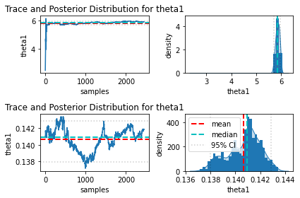
I also tried looking into parameters correlation and the trace, and I am also confused how to interpret them. If any of these supposed to help, I have attached them below as well (only part of the trace plot, because they seem to have similar trend like these, there were 2 chains, upper part for the first chain and lower part for the second one). The only thing that I noticed is that the behavior of these 2 chains are significantly different, but I do not know why.


theta0
theta1
theta2
theta3

Finally, if it helps, below is my model code:

    functions {
        real hill_activation(real x, real K, real n) {
            real hill;
            hill = pow(x, n) / (pow(K, n) + pow(x, n));
            return hill;
        }
        real growth_rate(real y, real a, real b) {
            real growth;
            growth = (a * (1 - (y/b)));
            return growth;
        }
        real[] gate_model(real t, real[] y, real[] theta, real[] x_r, int[] x_i) {
            
            real OD = y[1];
            real ECFn = y[2];
            real ECFc = y[3];
            real ECF = y[4];
            real GFP = y[5];
            real bn = theta[1];
            real bc = theta[2];
            real bg = theta[3];
            real syn_ECFn = theta[4];
            real syn_ECFc = theta[5];
            real syn_ECF = theta[6];
            real deg = theta[7];
            real syn_GFP = theta[8];
            real deg_GFP = theta[9];
            real K = theta[10];
            real n = theta[11];
            real alpha = x_r[1];
            real beta = x_r[2];
            int ind1 = x_i[1];
            int ind2 = x_i[2];
            real gamma = growth_rate(OD, alpha, beta);
            real dOD = gamma * OD;
            real dECFn = bn + syn_ECFn * ind1 - (deg + gamma) * ECFn;
            real dECFc = bc + syn_ECFc * ind2 - (deg + gamma) * ECFc;
            real dECF = syn_ECF * ECFn * ECFc - (deg + gamma) * ECF;
            real dGFP = bg + syn_GFP * hill_activation(ECF, K, n) - (deg_GFP + gamma) * GFP;
            return { dOD, dECFn, dECFc, dECF, dGFP };
        }
    }
    data {
        int<lower=1> T;
        int<lower=1> num_states;
        real y0[num_states];
        real y[T, 1];
        real t0;
        real ts[T];
        real od_params[2];
        int inducers[2];
    }
    transformed data {
        real x_r[2];
        int x_i[2];
        x_r[1] = od_params[1];
        x_r[2] = od_params[2];
        x_i[1] = inducers[1];
        x_i[2] = inducers[2];
    }
    parameters {
        real<lower=0> theta[11];
        real<lower=0> sigma;
    }
    model {
        real y_hat[T, num_states];
        theta[1] ~ uniform(0, 1e1);
        theta[2] ~ uniform(0, 1e1);
        theta[3] ~ uniform(0, 1e1);
        theta[4] ~ uniform(0, 1e2);
        theta[5] ~ uniform(0, 1e2);
        theta[6] ~ uniform(0, 1e-4);
        theta[7] ~ uniform(0, 1e-1);
        theta[8] ~ uniform(0, 1e0);
        theta[9] ~ uniform(0, 1e5);
        theta[10] ~ uniform(0, 1e2);
        theta[11] ~ uniform(0, 4);
        sigma ~ normal(0, 0.1);
        y_hat = integrate_ode_rk45(gate_model, y0, t0, ts, theta, x_r, x_i);
        y[,1] ~ normal(y_hat[,5], sigma);
    }

Thanks a lot.

the entries in theta seem to have very different prior scales, which may mean that the default initialization isn’t hitting them properly. Have you tried supplying manual inits at the center of those ranges? Alternatively, you could do:

...
    transformed data {
...
        array[11] real mults ; // n.b.
        mults[1] = 1e1 ;
        mults[2] = 1e1 ;
        mults[3] = 1e1 ;
        mults[4] = 1e2 ;
        mults[5] = 1e2 ;
        mults[6] = 1e-4 ;
        mults[7] = 1e-1 ;
        mults[8] = 1e0 ;
        mults[9] = 1e5 ;
        mults[10] = 1e2 ;
        mults[11] = 4 ;
  }
parameters {
        real<lower=0,multiplier=mults> theta[11]; // I *think* the multiplier syntax allows an array value
...    
}
...

Also, what’s the motivation for uniform priors (vs something that might achieve more gradual fall-off of credibility)?

1 Like

The uniform priors are simply because I have no idea about the behavior of the system that I modeled, so no assumption what other distribution I should use. Do you think I should try normal distribution instead?

As for the scales, I did point-based estimation before running MCMC (using curve_fit in Python), took the best estimate for each parameter, arbitrarily round them up slightly for the upper range, that is why the scales are quite different. I suspected that this is not a good approach, but I also have no idea how to initialize the parameters.

Can you elaborate what manual inits actually do? Or maybe point me to some reading material so that I can understand better? I definitely have not tried that. Because this is my first project dealing with parameter estimation (both with least square method or bayesian inference), I feel like I am quite blind and did a lot of try and error without any good reasons. I supposed my biggest problems are with the priors, and parameter initialization.

I think probably what will help you most is to start with a good book on linear regression and applied Bayesian modeling. If you have limited experience with regression (be it frequentist or Bayesian), Kruschke’s “Doing Bayesian Data Analysis” might be a good choice. I’ve also heard good things about @richard_mcelreath’s “Statistical Rethinking” and @andrewgelman, Hill, and @avehtari’s “Regression and other stories”.

1 Like

Building a principled prior model is a huge topic on its own. It may help to start by thinking about containment priors that just try to exclude extreme values; see for example Section 1.1.1.2 of Towards A Principled Bayesian Workflow. In particular what the natural units for the theta variables and how many orders of magnitude larger do the values have to be before they become weird?

That said the immediate problem here is that when using a bounded prior like the uniform your parameter bounds have to match or Stan will spend all of its time jumping into regions with zero prior mass. See for example the discussion in An Introduction to Stan.

The goal of Bayesian inference is to explore all model configurations consistent with the data and your domain expertise, not any single point estimate or the neighborhood immediately around a point estimate. Here your likelihood function, which encodes the model configurations consistent with the observed data, probably extends far past those scales estimated from the point estimate. In that case your heuristic priors would actually be excluding most of the model configurations that are consistent with the data and dramatically underestimating your uncertainties.

There is a lot more about all of these steps but hopefully by fixing the constraints or moving to a more reasonable prior model will get you going sooner rather than later.

1 Like