How to interpret estimated posterior distribution of hyperparameters returned by brms

[YidaZhang0628]

Hi, I am fitting a simple model with random effect as shown below:

alpha_i in the model represents random effect for different genes (i here represents genes). I assume alpha_i follows a normal distribution with a hierarchical prior sigma_gene. The ultimate goal is to estimate the posterior distribution of sigma_gene. Other variables are not related to this question so I skipped the introduction of them.

Here is how I specified prior for this model:

bpriors <- prior(normal(0, sigma_global_sd), class = "b", coef = "Intercept") +            
  prior(constant(1), class = "b", coef = "sc.prop") +                       
  prior(normal(0, sigma_gene_sd), class = "sd") +                           
  prior("target += cauchy_lpdf(sigma_global_sd | 0, 10)", check = FALSE) + 
  prior("target += cauchy_lpdf(sigma_gene_sd | 0, 10)", check = FALSE) +   
  prior(gamma(0.01, 0.01), class = "shape") +                              
  prior(beta(1, 1), class = "zi")                                           

stanvars <- stanvar(scode = "real<lower=0> sigma_global_sd; real<lower=0> sigma_gene_sd;",                                                      
                    block = "parameters")

sigma_gene_sd in the code represents sigma_gene in the model above. Below is the brms result after fitting the model:

Based on the result and the data I have, I am pretty sure that the distribution of sd_gene__Intercept represents the estimate posterior distribution of the hyperparameter sigma_gene in the model, i.e., the posterior distribution of the variance of the normal distribution of the random effect. Then my first question is, if this is correct, then what is the distribution for sigma_gene_sd? What is the difference between sd_gene__Intercept and sigma_gene_sd?

Another question is that, if I run prior_summary on the model, here are the list of parameters and their corresponding priors:

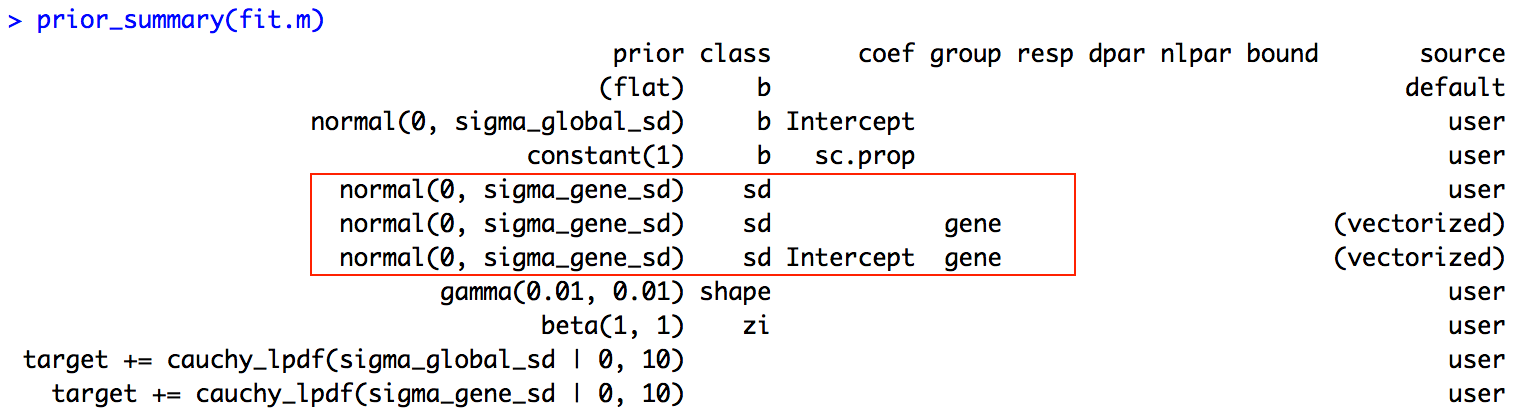
What is the difference between the three parameters in the red square? Are they three different parameters or they represent the same thing?

Thank you!

[YidaZhang0628]

Hi @paul.buerkner, not sure if you are the person to ask but since no one answers this question, I was wondering if I could get some directions from you?

[paul.buerkner]

The priors all mean the same here as you simply have one parameter. Prior specifiction brms is “hierarchical” in the way that the prior on the “more general” row will be vectorized to more specific cases if the specific cases don’t have priors themselves. For more details, see ?set_prior

With regard to your question about the SDs, I don’t know why you are manually adding these parameters. The one one alpha_i could be added via a random effect (1 | gene). The sigma_global as a hyperparameter seems strange to me as you simply have one parameter, alpha to inform that one (Imagine trying to estimate a standard deviation one just a single observation).

[YidaZhang0628]

Thank you for your response! Here are my answers and further questions based on your response:

1. I manually adding parameters like sigma_global_sd and sigma_gene_sd because I saw this post about hierarchical prior specification. I think my situation is the same as the example you showed in that post so I manually specified these hyperparameters. I tried to run with default prior and I am still able to get posterior distribution of b_Intercept and sd_gene__Intercept. Then my question is, is the result the same between default priors and manually specified hierarchical priors? It seems they are similar at least in my case. If that is true, then is there any advantage of using manually specified hierarchical priors? And for the hierarchical prior case, what is the meaning of the posterior distribution of sigma_gene_sd and sigma_global_sd in the plot output? It seems that these two are the two things that are not estimated if I use default prior.

2. For your concern of sigma_global_sd: I think this is the same as the point above. alpha is simply a global intercept. We can specify prior for it and estimate its posterior distribution. Here I simply give it a normal prior with standard deviation as sigma_global_sd. I can go without manually specifying it and the posterior distribution will still be estimated. So again, it comes back to the questions above, i.e., what is the difference between default priors and manually specified hierarchical priors.

[JLC]

Can you share your brms model syntax/specification? That might make it easier to see how the priors relate to model parameters.

[paul.buerkner]

specifying sigma_global_sd doesn’t make sense to me here. it will just follow its prior anyway so I would use a default prior in this case. I think you are making it unnecessarily complicated by estimating this hyperparameter.

you didn’t provide your brm() model specification so I am unsure how that looked but for the gene part right now. I recommend adding (1 | gene) which will add the desired hyperparamter automatically so you don’t need to fiddle with stanvars at all.

[YidaZhang0628]

Thanks! For sigma_global_sd, I will just remove it and use default prior.

Here is how I specify the model:

      fit.m <- brm(    
        bf(sp.count ~ 0 + Intercept + sc.prop + (1 | gene) + offset(log(cs))),           
        data = data2fit.all, 
        prior = bpriors, stanvars = stanvars,                                      # this line passes the prior & modified parameter blocks into brm()
        control = list(adapt_delta = 0.99, max_treedepth = 15),
        save_pars = save_pars(all = TRUE),                                                   
        family = zero_inflated_negbinomial(),
        iter = 2000, chains = 4, cores = 4
      )

bpriors and stanvars are provided at the beginning of my question. I think it is nothing but what you suggested, together with the manually specified priors. For the sake of simplicity, I will probably remove sigma_global_sd and sigma_gene_sd and use the default priors. Right now I am just trying to understand what difference would the hierarchical prior provide and how to interpret the additional parameters.

[YidaZhang0628]

I think the purpose of specifying those hierarchical priors explicitly is because I want the priors for both alpha and alpha_i to be normal distribution with mean 0 and unknown variance. In the default setting, the prior for alpha is flat and the prior for alpha_i is student_t(3, 0, 2.5). I have seen people simply using normal(0,10) as priors for intercept and random effect but I kind of don’t want to specify a fixed standard deviation (10 here). I think this is the main reason why I specify these hierarchical priors instead of using default priors.