Hierarchical Multivariate Ordinal Model Diagnostics (and tuning)

[JLC]

I am modelling data for 28 participants who rated “arousal” and “valence” using a combination pictographic (5 pictures) and Likert-type numeric (9-point) scale for each construct under 7 conditions: auditory only, audio-visual, low-pass filtered auditory only (half of the subjects (n = 14)), low-pass filtered auditory-visual (n = 14) high-pass filtered auditory only (half of the subjects (n = 14)), high-pass filtered auditory-visual (n = 14), and visual only (filtering not applicable). The stimuli consist of 65 “tokens” that have been categorized into “unpleasant”, “neutral”, “pleasant” - the number of tokens in each category is unbalanced.

So, it is a nested design, with half of the participants split on one sub-condition, and a bivariate response

I am trying to model the data as multivariate ordinal (cumulative(logit)).

I have uploaded the data here:
emo_modality_with_all_tokens.csv (609.3 KB)

My code for creating and running the model:

## List required packages ====
Pkgs <- c("tidyverse", "magrittr", "brms", 
           "rstan", "bayesplot",  
          "parallel",  "tidybayes")

### Load packages ====
lapply(Pkgs, require, c = T)

## Set computing options ====
ncores = detectCores()
rstan_options(auto_write = TRUE)
options(mc.cores = parallel::detectCores())

# Read in data ----
Modality_Ord <- read.csv("emo_modality_with_all_tokens.csv", stringsAsFactors = FALSE) %>%
        select("Subject" = ss_id, "Group" = filtering_group, "Filter" = filter_type,
               "Condition" = condition, "Category" = category_label,
               "Token" = token, "Arousal" = arousal, "Valence" = valence ) %>%
        mutate( Category = recode_factor(Category,
                                         unpleasant = "Unpleasant",
                                         neutral = "Neutral",
                                         pleasant = "Pleasant")) %>%
        droplevels() %>%
        mutate(Condition = ifelse(Condition == "fAO" | Condition == "fAV", 
                                  paste(Condition, Filter, sep = "_"), Condition),
               Subject = factor(Subject),
               Condition = factor(Condition, 
                                  levels = c("AO", "fAO_LP", "fAO_HP",
                                             "AV", "fAV_LP", "fAV_HP",
                                             "VO")),
               Token = factor(Token),
               Arousal = factor(Arousal, ordered = TRUE),
               Valence = factor(Valence, ordered = TRUE)) %>%
        select(-Group, -Filter) %>%
        ungroup() %>%
        na.omit()

## Multivariate model formula
Modality_ord_mv_fmla <- bf(mvbind(Arousal, Valence) ~ Category +
                                    Condition +
                                    Category:Condition +
                                    (1|o|Token) +
                                    (1|p|Condition) +
                                    (1|q|Condition:Subject))

## Specify priors
modality_ord_priors_mv <- c(
        set_prior("normal(0,2)",
                  class = "b",
                  resp = "Arousal"),
        
        set_prior("normal(0,6)",  
                  class = "Intercept",
                  coef = "",
                  resp = "Arousal"),
        
        set_prior("normal(0,0.125)",
                  class = "sd",
                  coef = "Intercept",
                  group = "Condition",
                  resp = "Arousal"),
        set_prior("normal(0,0.125)",
                  class = "sd",
                  coef = "Intercept",
                  group = "Condition:Subject",
                  resp = "Arousal"),
        set_prior("normal(0,0.125)",
                  class = "sd",
                  coef = "Intercept",
                  group = "Token",
                  resp = "Arousal"),
        
        set_prior("normal(0,2)",
                  class = "b",
                  resp = "Valence"),
        
        set_prior("normal(0,6)",  
                  class = "Intercept",
                  coef = "",
                  resp = "Valence"),
        
        set_prior("normal(0,0.125)",
                  class = "sd",
                  coef = "Intercept",
                  group = "Condition",
                  resp = "Valence"),
        set_prior("normal(0,0.125)",
                  class = "sd",
                  coef = "Intercept",
                  group = "Condition:Subject",
                  resp = "Valence"),
        set_prior("normal(0,0.125)",
                  class = "sd",
                  coef = "Intercept",
                  group = "Token",
                  resp = "Valence")
)

# Compile and fit model 
Modality_Ord_MV_Mod <-
        brm(Modality_ord_mv_fmla,
            data = Modality_Ord,
            family = cumulative("logit"),
            prior = modality_ord_priors_mv,
            inits = 0,
            iter = 2000,
            warmup = 1000,
            chains = 2,
            cores = ncores,
            sample_prior = TRUE,
            save_all_pars = TRUE,
            control = list(adapt_delta = 0.99,
                           max_treedepth = 12)
        )

The model seems to converge fairly efficiently and the fits to the data for both responses seem good:

Arousal:
pp_check(Modality_Ord_MV_Mod, resp = "Arousal")

Valence:
pp_check(Modality_Ord_MV_Mod, resp = "Valence")

I am seeing some poor PSIS-LOO checks, however:

Looking at Arousal:

loo_mv_arl <- loo(Modality_Ord_MV_Mod, resp = "Arousal", 
                            save_psis = TRUE)

yrep_arl <- posterior_predict(Modality_Ord_MV_Mod, resp = "Arousal")

ppc_loo_pit_overlay(
        y = as.numeric(Modality_Ord$Arousal),
        yrep = as.matrix(yrep_arl),
        lw = weights(loo_mv_arl$psis_object)
)

Looking at Valence

loo_mv_val <- loo(Modality_Ord_MV_Mod, resp = "Valence", 
                  save_psis = TRUE)

yrep_val <- posterior_predict(Modality_Ord_MV_Mod, resp = "Valence")

ppc_loo_pit_overlay(
        y = as.numeric(Modality_Ord$Valence),
        yrep = as.matrix(yrep_val),
        lw = weights(loo_mv_val$psis_object)
)

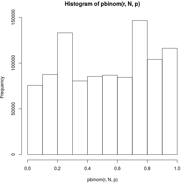
My understanding is that the LOO PITs should be uniform for continuous data; does that apply if the the model is based on a continuous latent variable rather than a true continuous response?

Does this suggest the model is over-dispersed for both responses?

How might I go about further generalizing the model to account for the abundance of large errors?

Would adding a distribution over the disc parameter be of any help?

Edit: I tried adding disc to the model and saw no change in LOO-PIT.

[martinmodrak]

Sorry, your question fell through despite being relevant and well written.

A small suggestion I have is that for ordinal data, ppc_bars will produce clearer output than ppc_dens.

@JLC

My understanding is that the LOO PITs should be uniform for continuous data; does that apply if the the model is based on a continuous latent variable rather than a true continuous response?

Does this suggest the model is over-dispersed for both responses?

How might I go about further generalizing the model to account for the abundance of large errors?

I have very little experience with PSIS-LOO plots, but I’ll take a guess that the plot tells you that your data are more likely to be found above the median of the leave-one-out predictive distribution than below, i.e. there is a skew towards higher values that is not captured by the model.

However, since your overall pp_checks look good, it might be possible this is because the model actually overfits the data. But first, I would suggest you do some grouped pp checks (e.g. type = "bars_grouped") slicing the data by various categories using the group parameter as this may also show some discrepancies.

I know @avehtari is busy, but hope he can check my reasoning here.

[JLC]

Thank you, Martin!

I’ll look a little further with some bar plots and will share my results here.

[avehtari]

PPC looks marginal distribution, while LOO-PIT looks at the conditional distributions and thus there can be a big difference in the results.

@JLC

My understanding is that the LOO PITs should be uniform for continuous data; does that apply if the the model is based on a continuous latent variable rather than a true continuous response?

For discrete data see Predictive Model Assessment for Count Data. If there are many unique values in discrete space the issue is smaller. This is something we should fix for LOO-PIT plots, but the progress has been delayed by thinking more about how to present the deviation from uniformity better than the current approach.

[martinmodrak]

So if I understand you correctly, the current implementation of the PIT in the bayesplot package doesn’t expect ties in data and if you want to use the LOO-PIT checks for discrete data, you need to compute the PIT yourself, using the approach in the linked paper. Is that correct?

[avehtari]

@martinmodrak

So if I understand you correctly, the current implementation of the PIT in the bayesplot package doesn’t expect ties in data

It’s not about ties, but about 1) whether we compute ecdf with < or <= and 2) that values in discrete case have a finite number of discrete values that are not uniformly distributed. Case 2) is illustrated in the example below

n<-1000000;N<-100;p<-.3;r<-rbinom(n, N, p);
hist(pbinom(r, N, p), breaks=1000)

Note that I intentionally had 1000 bins. The issue is that this can be sensitive to the number and placement of bins, but with 10 bins we get

hist(pbinom(r, N, p), breaks=10)

but this is skewed to right

A quick approximation to correct is to use midpoint between < and <=

hist(0.5*pbinom(r-1, N, p)+0.5*pbinom(r, N, p), breaks=10)

The randomized PIT is

hist(pbinom(r-1, N, p)+runif(n)*(pbinom(r, N, p)-pbinom(r-1, N, p)), breaks=1000)

which looks uniform even with 1000 breaks.

So the current version is doing something wrong for discrete, but how much wrong depends on the case and number of bins in histogram or kernel width in the kernel density estimate. The above mentioned paper has correct non-randomized version which would be nice to have, but it’s been a resource issue to get it done.

[JLC]

My apologies for the delay in getting back to this thread. Thank you all for the valuable lessons and input!

I created some grouped bar pp_checks for each response, grouped first by condition, and then by stimulus category. To me, it looks like the model is doing a fairly good job, but I would very much appreciate any input on how I can further diagnose the model before we submit for publication.

Arousal by Condition:

Arousal by Category:

Valence by Condition:

Valence by Category:

[martinmodrak]

Hi, I kind of missed this, so getting back after a while.

The plots don’t look terrible, but they also don’t look great. It appears that in many cases, there is some issue with the item 5 not being predicted very well.

Also, both the “by Category” plots have quite a lot of the posterior intervals missing the data.

I think both should warrant at least some additional investigation. Is there a reason why 5 might be special?

In particular, the most useful pp checks tend to be by splitting on category that is NOT included in your model. Say, the order the question was displayed. Or any other covariate you did record bu have not used. Also using the “stat_grouped” might be useful for some statistic that the model doesn’t directly model - say sd of the answers. Or computing the maximum and minimum of answers per subject (having this PP check will likely require some additional processing code on your side)

But since we see problems already with grouping you have included in the model, one possibility is that you priors for the sd parameters are too narrow… Does the posterior for the sd parameters “fight” the prior? (i.e. the sd priors would put most of the mass below roughly 0.125 * 2 = 0.25, if the posterior 95% interval includes 0.25 it is a hint that the prior might be substantially influencing the posterior).

Does that make sense? Best of luck with the publication!

[JLC]

Thank you @martinmodrak!

I’ll do some further interrogation of the model.

For the priors on the sd parameters, my thinking was that since I am using a logit link, that I’d be putting most of the mass below exp(0.125*2) = 1.65. All of the posterior intervals have an upper limit below 1, so I thought I might be safe there.

Do only beta priors also use logit link, or does the link function apply to sd parameters as well?

[martinmodrak]

The link function applies to the complete linear predictor (sum of intercept and all effect terms). The sd_XXX parameters (and all others) are reported in the model summary on the log odds scale.

@JLC

For the priors on the sd parameters, my thinking was that since I am using a logit link, that I’d be putting most of the mass below exp(0.125*2) = 1.65.

Note that you are putting most of the mass of the sd parameter below 0.125 * 2, which in turn means that most of the varying intercepts will be within +/- ((0.125) * 2) * 2 = +/- 0.5 (this is an overestimate - it is unlikely that both sd AND the varying intercept are at the extreme tail at once, but it works for rough checks), so most of the varying intercepts will end up multiplying/dividing the (non-log) odds by at most exp(0.5).

Does that make sense?

[JLC]

Thank you very much, Martin! Your explanation both makes sense and helps tremendously!

All of the support in this thread helped me realize not only does my model need further interrogation, but also my data partitioning.

In examining the counts of responses per token, it’s appears the “Categories” have very heterogeneous ratings. As an example, these are the distributions of responses per token, by category, for a single condition:

To me this suggests two possible strategies: i) broad parameterization of variance within category, or ii) re-partitioning of the data into categories supported by behavioural responses.

I plan to try both strategies!

[JLC]

As @martinmodrak suggested, I looked deeper into where my variance could expanded and ended up putting some broader priors on the subject-level sd’s. This seems to have helped the fit and predictions quite a bit:

Subject level:

Stimulus (token) level:

Category:

Condition:

[JLC]

As we get these data ready for the final push to publication, I wanted to create some plots similar to Liddell & Kruschke (2018)

[martinmodrak]

Yes, this looks quite a bit better. But what is happening with response 5? It looks like it is driving a lot (if not all) of the remaining discrepancies… Was that a likert scale with 9 items where 5 is neutral?

Maybe this is still some issue with the priors - could you show the result of summary for the fit?

Alternatively (and this is just a guess) you might get better results with sequential (cratio/sratio) or adjacent category (acat) ordinal regressions (see https://psyarxiv.com/x8swp/ for explanation of those)

[JLC]

Thanks, Martin!

Yes, this was a 9 item likert with 5 as neutral.

I set the priors as follows:

## Set priors
priors_mv <- c(
        set_prior("normal(0,6)",  
                  class = "Intercept",
                  coef = "",
                  group = "Neutral", 
                  resp = "Arousal"),
        
        set_prior("normal(0,6)",  
                  class = "Intercept",
                  coef = "",
                  group = "Pleasant",
                  resp = "Arousal"),
        
        set_prior("student_t(6,1,1.5)",
                  class = "b",
                  coef = "",
                  resp = "Arousal"),
        
        set_prior("normal(0,2)",
                  class = "b",
                  coef = "CategoryNeutral",
                  resp = "Arousal",
                  dpar = "disc"),
        
        set_prior("normal(0,2)",
                  class = "b",
                  coef = "CategoryPleasant",
                  resp = "Arousal",
                  dpar = "disc"),
        
        set_prior("exponential(2)",
                  class = "sd",
                  coef = "Intercept",
                  group = "Condition",
                  resp = "Arousal"),
        set_prior("exponential(3)",
                  class = "sd",
                  coef = "Intercept",
                  group = "Condition:Subject",
                  resp = "Arousal"),
        set_prior("exponential(2)",
                  class = "sd",
                  coef = "Intercept",
                  group = "Token",
                  resp = "Arousal"),
        
        set_prior("normal(0,6)",  
                  class = "Intercept",
                  coef = "",
                  group = "Neutral", 
                  resp = "Valence"),
        
        set_prior("normal(0,6)",  
                  class = "Intercept",
                  coef = "",
                  group = "Pleasant",
                  resp = "Valence"),
        
        set_prior("student_t(6,1,1.5)",
                  class = "b",
                  coef = "",
                  resp = "Valence"),
        
        set_prior("normal(0,2)",
                  class = "b",
                  coef = "CategoryNeutral",
                  resp = "Valence",
                  dpar = "disc"),
        
        set_prior("normal(0,2)",
                  class = "b",
                  coef = "CategoryPleasant",
                  resp = "Valence",
                  dpar = "disc"),
        
        set_prior("exponential(2)",
                  class = "sd",
                  coef = "Intercept",
                  group = "Condition",
                  resp = "Valence"),
        set_prior("exponential(3)",
                  class = "sd",
                  coef = "Intercept",
                  group = "Condition:Subject",
                  resp = "Valence"),
        set_prior("exponential(2)",
                  class = "sd",
                  coef = "Intercept",
                  group = "Token",
                  resp = "Valence")
)

Here is the summary of the fit:

 Family: MV(cumulative, cumulative) 
  Links: mu = probit; disc = log
         mu = probit; disc = log 
Formula: Valence | resp_thres(8, gr = Category) ~ Category + Condition + Category:Condition + Intensity.c + (1 | o | Token) + (1 | p | Condition) + (1 | q | Condition:Subject) 
         disc ~ 0 + Category
         Arousal | resp_thres(8, gr = Category) ~ Category + Condition + Category:Condition + Intensity.c + (1 | o | Token) + (1 | p | Condition) + (1 | q | Condition:Subject) 
         disc ~ 0 + Category
   Data: Modality_Ord_Full (Number of observations: 6516) 
Samples: 4 chains, each with iter = 4000; warmup = 1500; thin = 1;
         total post-warmup samples = 10000

Group-Level Effects: 
~Condition (Number of levels: 7) 
                                         Estimate Est.Error l-95% CI u-95% CI Rhat Bulk_ESS Tail_ESS
sd(Valence_Intercept)                        0.39      0.32     0.01     1.19 1.00     2190     4105
sd(Arousal_Intercept)                        0.33      0.29     0.01     1.06 1.00     2173     3390
cor(Valence_Intercept,Arousal_Intercept)     0.11      0.57    -0.93     0.96 1.00     4801     6040

~Condition:Subject (Number of levels: 140) 
                                         Estimate Est.Error l-95% CI u-95% CI Rhat Bulk_ESS Tail_ESS
sd(Valence_Intercept)                        0.41      0.03     0.35     0.48 1.00     3306     5443
sd(Arousal_Intercept)                        0.46      0.04     0.39     0.53 1.00     2512     4590
cor(Valence_Intercept,Arousal_Intercept)    -0.48      0.08    -0.63    -0.31 1.00     2140     4848

~Token (Number of levels: 51) 
                                         Estimate Est.Error l-95% CI u-95% CI Rhat Bulk_ESS Tail_ESS
sd(Valence_Intercept)                        1.11      0.17     0.82     1.47 1.00      920     2518
sd(Arousal_Intercept)                        0.93      0.12     0.71     1.20 1.00     1251     2680
cor(Valence_Intercept,Arousal_Intercept)    -0.61      0.10    -0.78    -0.41 1.00     1830     3291

Population-Level Effects: 
                                         Estimate Est.Error l-95% CI u-95% CI Rhat Bulk_ESS Tail_ESS
Valence_Intercept[Unpleasant,1]             -0.86      0.47    -1.65     0.20 1.00     1178     2150
Valence_Intercept[Unpleasant,2]             -0.02      0.47    -0.81     1.05 1.00     1180     2096
Valence_Intercept[Unpleasant,3]              0.69      0.47    -0.09     1.75 1.00     1178     2071
Valence_Intercept[Unpleasant,4]              1.40      0.47     0.62     2.47 1.00     1187     2164
Valence_Intercept[Unpleasant,5]              2.19      0.47     1.42     3.27 1.00     1189     2040
Valence_Intercept[Unpleasant,6]              2.56      0.47     1.79     3.64 1.00     1198     2182
Valence_Intercept[Unpleasant,7]              2.98      0.47     2.19     4.05 1.00     1219     2178
Valence_Intercept[Unpleasant,8]              3.41      0.48     2.61     4.48 1.00     1244     2159
Valence_Intercept[Neutral,1]                -5.33      1.80    -9.02    -1.98 1.00     1433     3277
Valence_Intercept[Neutral,2]                -3.67      1.60    -6.88    -0.70 1.00     1903     4115
Valence_Intercept[Neutral,3]                -1.88      1.44    -4.76     0.83 1.00     3412     5710
Valence_Intercept[Neutral,4]                -0.57      1.38    -3.34     2.06 1.00     6568     6649
Valence_Intercept[Neutral,5]                 1.56      1.37    -1.21     4.19 1.00     8020     7219
Valence_Intercept[Neutral,6]                 2.98      1.45     0.09     5.78 1.00     5285     6544
Valence_Intercept[Neutral,7]                 4.35      1.57     1.26     7.40 1.00     3269     4845
Valence_Intercept[Neutral,8]                 5.87      1.74     2.53     9.38 1.00     2253     3462
Valence_Intercept[Pleasant,1]               -8.58      1.87   -12.39    -5.00 1.00     1758     3443
Valence_Intercept[Pleasant,2]               -5.86      1.62    -9.13    -2.69 1.00     2406     4321
Valence_Intercept[Pleasant,3]               -4.04      1.49    -6.96    -1.08 1.00     3347     5001
Valence_Intercept[Pleasant,4]               -2.16      1.40    -4.87     0.67 1.00     5119     6324
Valence_Intercept[Pleasant,5]                0.12      1.34    -2.45     2.91 1.00     8050     6362
Valence_Intercept[Pleasant,6]                2.18      1.36    -0.43     5.00 1.00     6964     6003
Valence_Intercept[Pleasant,7]                4.30      1.43     1.56     7.31 1.00     4153     5330
Valence_Intercept[Pleasant,8]                6.95      1.60     3.90    10.24 1.00     2459     4110
Arousal_Intercept[Unpleasant,1]             -2.69      0.40    -3.35    -1.75 1.00     1535     2174
Arousal_Intercept[Unpleasant,2]             -2.19      0.40    -2.84    -1.26 1.00     1521     2073
Arousal_Intercept[Unpleasant,3]             -1.86      0.40    -2.51    -0.91 1.00     1514     2125
Arousal_Intercept[Unpleasant,4]             -1.48      0.40    -2.13    -0.55 1.00     1503     2099
Arousal_Intercept[Unpleasant,5]             -0.44      0.40    -1.08     0.49 1.00     1491     2104
Arousal_Intercept[Unpleasant,6]              0.41      0.40    -0.23     1.33 1.00     1492     2101
Arousal_Intercept[Unpleasant,7]              1.21      0.40     0.55     2.13 1.00     1492     2150
Arousal_Intercept[Unpleasant,8]              1.99      0.40     1.34     2.93 1.00     1501     2108
Arousal_Intercept[Neutral,1]                -4.23      1.58    -7.49    -1.23 1.00     3080     4743
Arousal_Intercept[Neutral,2]                -2.84      1.47    -5.84     0.03 1.00     4210     5472
Arousal_Intercept[Neutral,3]                -1.60      1.40    -4.45     1.13 1.00     5978     6188
Arousal_Intercept[Neutral,4]                -0.50      1.36    -3.26     2.12 1.00     7519     6315
Arousal_Intercept[Neutral,5]                 1.87      1.35    -0.82     4.45 1.00     8646     6554
Arousal_Intercept[Neutral,6]                 3.51      1.41     0.69     6.26 1.00     6708     6315
Arousal_Intercept[Neutral,7]                 5.24      1.52     2.26     8.23 1.00     3987     5620
Arousal_Intercept[Neutral,8]                 7.23      1.70     3.96    10.71 1.00     2756     4129
Arousal_Intercept[Pleasant,1]               -3.26      1.39    -6.04    -0.59 1.00     4695     6074
Arousal_Intercept[Pleasant,2]               -2.10      1.35    -4.81     0.51 1.00     5772     6428
Arousal_Intercept[Pleasant,3]               -1.19      1.34    -3.88     1.40 1.00     6418     6307
Arousal_Intercept[Pleasant,4]               -0.50      1.32    -3.16     2.08 1.00     6780     6275
Arousal_Intercept[Pleasant,5]                0.90      1.32    -1.77     3.45 1.00     7197     6141
Arousal_Intercept[Pleasant,6]                2.05      1.32    -0.64     4.64 1.00     7073     6161
Arousal_Intercept[Pleasant,7]                3.41      1.35     0.70     6.03 1.00     6378     6066
Arousal_Intercept[Pleasant,8]                4.84      1.39     2.04     7.55 1.00     5366     6086
Valence_CategoryNeutral                      0.73      1.33    -1.96     3.31 1.00    10772     7029
Valence_CategoryPleasant                     1.48      1.32    -1.10     4.22 1.00     9454     6062
Valence_ConditionfAO_LP                      0.60      0.59    -0.37     2.06 1.00     3075     3723
Valence_ConditionfAO_HP                      0.53      0.59    -0.37     2.04 1.00     2898     3835
Valence_ConditionAV                          0.03      0.60    -0.85     1.60 1.00     2848     3741
Valence_ConditionfAV_LP                      0.06      0.60    -0.83     1.58 1.00     3022     4404
Valence_ConditionfAV_HP                      0.07      0.61    -0.86     1.57 1.00     2807     3643
Valence_ConditionVO                          0.49      0.57    -0.40     1.91 1.00     3042     3989
Valence_Intensity.c                         -0.21      0.03    -0.27    -0.15 1.00    12121     6965
Valence_CategoryNeutral:ConditionfAO_LP     -0.54      0.32    -1.18     0.10 1.00     6359     4860
Valence_CategoryPleasant:ConditionfAO_LP    -2.41      0.37    -3.23    -1.74 1.00     1945     3921
Valence_CategoryNeutral:ConditionfAO_HP     -1.43      0.37    -2.20    -0.73 1.00     6161     6089
Valence_CategoryPleasant:ConditionfAO_HP    -1.75      0.33    -2.45    -1.15 1.00     3491     5072
Valence_CategoryNeutral:ConditionAV          0.70      0.29     0.17     1.31 1.00     3751     3796
Valence_CategoryPleasant:ConditionAV         1.91      0.32     1.33     2.61 1.00     1738     3833
Valence_CategoryNeutral:ConditionfAV_LP      0.53      0.33    -0.08     1.23 1.00     4352     4517
Valence_CategoryPleasant:ConditionfAV_LP     0.50      0.29    -0.06     1.09 1.00     6192     6140
Valence_CategoryNeutral:ConditionfAV_HP     -0.11      0.36    -0.78     0.62 1.00     6639     4985
Valence_CategoryPleasant:ConditionfAV_HP    -0.44      0.30    -1.05     0.12 1.00     8897     6447
Valence_CategoryNeutral:ConditionVO          0.27      0.29    -0.25     0.92 1.00     3586     3971
Valence_CategoryPleasant:ConditionVO         1.52      0.33     0.93     2.22 1.00     1673     3249
disc_Valence_CategoryNeutral                -0.86      0.21    -1.27    -0.47 1.01      766     1856
disc_Valence_CategoryPleasant               -1.26      0.14    -1.54    -0.99 1.00      925     2135
Arousal_CategoryNeutral                      0.41      1.32    -2.32     2.90 1.00     9531     6155
Arousal_CategoryPleasant                     0.67      1.31    -1.97     3.19 1.00     7302     5992
Arousal_ConditionfAO_LP                     -0.03      0.52    -0.86     1.29 1.00     2934     2759
Arousal_ConditionfAO_HP                      0.29      0.53    -0.56     1.61 1.00     3028     3207
Arousal_ConditionAV                          0.42      0.50    -0.41     1.67 1.00     2546     2664
Arousal_ConditionfAV_LP                      0.46      0.52    -0.40     1.74 1.00     2818     3228
Arousal_ConditionfAV_HP                      0.47      0.53    -0.42     1.77 1.00     2828     2708
Arousal_ConditionVO                         -0.09      0.53    -0.92     1.25 1.00     2728     2669
Arousal_Intensity.c                          0.29      0.03     0.24     0.35 1.00    12607     6847
Arousal_CategoryNeutral:ConditionfAO_LP      0.15      0.31    -0.48     0.75 1.00     7615     6317
Arousal_CategoryPleasant:ConditionfAO_LP    -0.44      0.19    -0.84    -0.09 1.00     2491     3897
Arousal_CategoryNeutral:ConditionfAO_HP      1.21      0.36     0.55     1.93 1.00     6479     6151
Arousal_CategoryPleasant:ConditionfAO_HP    -0.06      0.17    -0.41     0.27 1.00     5354     6636
Arousal_CategoryNeutral:ConditionAV         -0.41      0.27    -0.94     0.11 1.00     7561     7098
Arousal_CategoryPleasant:ConditionAV        -0.14      0.13    -0.40     0.11 1.00     8272     7264
Arousal_CategoryNeutral:ConditionfAV_LP     -0.69      0.33    -1.36    -0.08 1.00     5869     5634
Arousal_CategoryPleasant:ConditionfAV_LP    -0.65      0.17    -1.02    -0.33 1.00     3489     5215
Arousal_CategoryNeutral:ConditionfAV_HP      0.59      0.35    -0.08     1.29 1.00     8534     6300
Arousal_CategoryPleasant:ConditionfAV_HP    -0.11      0.17    -0.44     0.22 1.00     6896     6170
Arousal_CategoryNeutral:ConditionVO         -0.17      0.28    -0.75     0.34 1.00     6019     5620
Arousal_CategoryPleasant:ConditionVO        -0.29      0.15    -0.59    -0.02 1.00     3439     4802
disc_Arousal_CategoryNeutral                -0.86      0.16    -1.19    -0.56 1.00     1036     2662
disc_Arousal_CategoryPleasant               -0.58      0.11    -0.80    -0.37 1.00     1149     2531

Samples were drawn using sampling(NUTS). For each parameter, Bulk_ESS
and Tail_ESS are effective sample size measures, and Rhat is the potential
scale reduction factor on split chains (at convergence, Rhat = 1).

[martinmodrak]

Overall, I would just try if anything changes if you run the model with priors two or three times as wide. The exponential priors for sd are a bit unusual, but not obviously wrong. exponential(2) should mean that 95% of the prior mass is on sd < 1.5, and for exponential(3) on sd < 1. So I think they could still be influencing the posterior at least for sd(Valence_Intercept) which touches on that soft boundary.

I also think it is weird that your prior for class = "b", resp = "Arousal" is not centered at zero - do you have good reasons to a priori expect those to be positive?

The fact that many responses have quite abundant the neutral response is also a potential warning that there might be something wrong with the experiment design - e.g. people not really understanding what they are supposed or not really engaging with the experiment could lead them to prefer the neutral option… This would mean you have a separate process generating part of those response, which you may need to model…

[JLC]

Thank you once again, Martin!

I’m re-running now with broader priors (exp(0.5) and centering the betas at 0.

There are definitely some concerns with the design and the stimuli. Many of the neutral responses were expected and intended in the “neutral” category of stimuli.

I am unsure how to approach modelling a separate process for the neutral responses; would that be an addition to the current model, or a separate model for just those responses? Are there any resources or reference you could direct me toward?

[martinmodrak]

@JLC

I am unsure how to approach modelling a separate process for the neutral responses; would that be an addition to the current model, or a separate model for just those responses? Are there any resources or reference you could direct me toward?

Unfortunately, I don’t think there is an easy and straightforward solution. One hack would be to define a predictor is_neutral that would be 1 when the response is neutral and 0 otherwise. You could then use is_neutral in your formula by itself or even as interaction, so say Category:is_neutral would end up adding another effect of Category only for neutral responses. This way, you get additional flexibility in the model only for the neutral category. Interpreting such coefficients directly would however be quite tricky.

A better way would be to define a custom “5 - inflated ordinal” response family that would have one additional parameter for the degree of 5 inflation (that you can then put predictors on). This is semi-advanced, but has been done before, see: Ordinal Mixture Model w/ Set Outcome for One Component - #20 by mike-lawrence (the code there is unfortunately incomplete) and there is some semi-related discussion at Test zero inflated Graded response model

Does that make sense?

[JLC]

Thank you, Martin! That does make sense!