Guidance on prior predictive checks in ordinal model

[natpac]

Hello,
Sorry in advance for the long post…
I am working to fit an ordinal logistic regression with brms to species’ risk extinction categories (ranging in order from Low to High risk : 5 levels) vs several predictors (numeric, nominal, ordered; ecological characteristics). I have around 100 observations, but some levels are not observed in all extinction categories.
I have read quite a lot of posts here and some other docs but I would like some guidance as I have trouble making sense of the prior predictive checks and model checking. I have no real a priori of what the Intercept thresholds or predictor relations should be.
My final aim is to use the package projpred to do some predictor selection as I expect that some factors may be redundant.

---

Starting with the NULL model below:

brm(
  formula = extinction_cat ~ 1
  , data = df_extinction
  , family = cumulative("logit")
  # , sample_prior = 'only'
  , iter = 18000
  , warmup = 12000
  , thin = 3
  , chains = 3
  , cores = 3
)

I get prior-data conflict on one of the Intercept with priorsense::powerscale_sensitivity

I get these posterior pp_check

And this when I run it with sample_prior = 'only':

I found that using slightly weaker prior prior = c(prior(student_t(3, 0, 5), class = "Intercept")) remove the prior-data conflict but seems to increase the dome-shaped of the pp_check.

(1) Is this the right decision?

---

Then I add one nominal predictor to the model. This predictor is not really well distributed in each extinction categories and two levels have low observation count and only in one extinction category (only 2 species in level C, and 4 in F).

When checking the posteriors, one dietC has a large distribution and powerscale_sensitivity indicates a weak likelihood (which I guess makes sense as there is not a lot of info in the observations).

bars_grouped pp_check:

(2) Why is dietC completely off? And why dietF isn’t then?

---

As prior_sample = “only” doesn’t work with the default priors, I set the prior of b to the same weakly informative prior as for the Intercept student_t(3, 0, 5) which reduce the uncertainty in dietC but the weak likelihood is still there (and pp_check looks the same).

with sample_prior = 'only':

With power scaling sensitivity (powerscale_plot_ecdf) :

If I precise the priors on b student_t(3, 0, 2.5), it goes to prior-data conflict

(3) Not sure what the solution is here for the final model between choosing prior-data conflict or weak likelihood.

---

Thanks for your help!

---

• Operating System: Windows
• brms Version: 2.20.4
• priorsense Version: 0.0.0.9

[harrelfe]

Side comment: variable selection is generally not a good idea. For one thing your sample size is too small by a factor of 100 to reliably tell you which predictors are important. Secondly the resulting posterior distributions will be too narrow unless you are using shrinkage priors to do all the work of predictor selection.

[natpac]

Thank you for the information!
I wanted to keep the variable selection for another post maybe but might as well discuss it now. I know that variable selection is not the best but the recent development of the projpred package seems like a really good step forward!
(1) On your comment:

your sample size is too small by a factor of 100

Can you specify what you are referring to? (number of observation vs number of predictor?) What is the required sample size ?

You are suggesting to use shrinkage prior.
(2) I remember seeing a post where avehtari said something about a required minimum number of covariates for shrinkage prior to be useful. I have around 10 covariates. Any comment on that?
(3) Would this be the right way of coding a shrinkage prior?
prior = c(prior(horseshoe(1), class = "b")
And then maybe play with the par_ratio argument?
(4) Is there anything to tweak given that I will have numeric, nominal and ordered predictors?
(5) I saw multiple posts on horseshoe prior resulting in different (greater) shrinkage compared to some other methods of variable selection. Any suggestions?

---

Any comment on the questions of the original post?

[avehtari]

@harrelfe

Side comment: variable selection is generally not a good idea. For one thing your sample size is too small by a factor of 100 to reliably tell you which predictors are important.

@natpac

Can you specify what you are referring to? (number of observation vs number of predictor?) What is the required sample size ?

I disagree with Frank, as the required sample size depends on the signal-noise-ratio, observation model, priors, variable selection method, the goal of the variable selection, and what is meant by reliably. It is possible to do useful variable selection also when the number of observations is smaller than the number of variables. A good variable selection approach also tells if the sample size is not big enough, and specifically does not perform worse than using the full model (like projpred). Use of good priors is important also for the full model.

@natpac

(2) I remember seeing a post where avehtari said something about a required minimum number of covariates for shrinkage prior to be useful. I have around 10 covariates. Any comment on that?

10 is a small number considering sparsity assumption, but if you know that only 1 or 2 covariates are likely to have bigger effects, then sparsity prior is appropriate. Now days I would use R2D2 style prior which sets the prior on total explanation power and it’s easier to specify than horseshoe in case of small number of covariates that may all have weak effect or that may be correlating. The development of R2D2 style priors for non-normal families is still in progress, but the specification seems to be that way robust that you can get good results even if you would use it as for normal model, that is, prior = prior(R2D2(), class="b") and maybe play with mean_R2 and prec_R2 parameters (I usuallay start with mean_R2 = 1/3, prec_R2 = 3)

@natpac

(4) Is there anything to tweak given that I will have numeric, nominal and ordered predictors?

That is a challenge, and I don’t have a research based answer, but you can try and use priorsense package to assess prior-likelihood-sensitivity.

@natpac

(5) I saw multiple posts on horseshoe prior resulting in different (greater) shrinkage compared to some other methods of variable selection. Any suggestions?

Priors and variable selection are separate things. Priors are information about the assumed effect sizes. Variable selection is decision-making about which variables to use (and which can be fixed to 0) and how to make the inference after the selection.

[harrelfe]

As the original poster stated, your projection method of variable selection is the most promising approach. I was referring to ordinary variable selection, with the typical low S:N ratio I see in biomedical research, in which case I stand by my statement that an enormous sample size is needed to come close to having a good probability of selection of the “right” predictors. I also have doubts that an N < p case has a decent probability of selecting the right variables, even when allowing for some non-overlap in the sets and not demanding exactly correct selection.

[natpac]

Thank you avehtari for your guidance!

I ran the full model (11 covariates of multiple types) with R2D2 priors on b with :

• prior(R2D2(mean_R2 = 1/3, prec_R2 = 3), class = "b")

… leading to prior-data conflict on half of all parameters

Most covariates posteriors are centered around 0, but some might have a slight or noticeable effect:

Good overall posterior pp_check but maybe two problematic specific posterior pp_check:

• and default brms parameters : prior(R2D2(mean_R2 = 1/2, prec_R2 = 2), class = "b")

that raised less prior-data conflict:

but gave very similar summary output and pp_check.

---

(1) You said to “play” a bit with the parameters, and I tested a bunch of other combinations but is there a guideline on what a good value could be ?

(2) I am still not sure how to resolve the prior check issue with powerscale_sensitivity, if it is really an issue (given that the pp_check look good) ?

[avehtari]

@natpac

leading to prior-data conflict on half of all parameters

Some of these parameters are weakly identified and conflict is not real. Focus on the quantity of interest (can also be prediction). Do you see conflict for that?

@natpac

(1) You said to “play” a bit with the parameters, and I tested a bunch of other combinations but is there a guideline on what a good value could be ?

The question is does the posterior or prediction for the quantity of interest change substantially if you change the prior.

[avehtari]

Adding a link to a notebook with several examples on using priorsense with focus on different quantities of interest Bayesian data analysis - BRMS demos

[n-kall]

@natpac

• and default brms parameters : prior(R2D2(mean_R2 = 1/2, prec_R2 = 2), class = "b")

that raised less prior-data conflict:

Small note: The default brms parameters for the R2D2 prior result in a uniform prior on R2. priorsense requires non-uniform priors in order for the power-scaling to have an effect. This is likely why the prior sensitivity is lower in this model.

[natpac]

Thank you both very much for your time! The Priorsense package and the R2D2 prior are quite new to me and I am still a bit confused on how to use them properly .

The powerscale_plot_ecdf plots below (based on prior(R2D2(mean_R2 = 1/3, prec_R2 = 3), class = "b")) do not show a lot of prior sensitivity:

Although I did not find how to estimate what values of mean_R2 and prec_R2 are tested by the power-scaling sensitivity given alpha from 0.8 to 1.25. This and, your post, avehtari, and n-kall’s comment make me wonder how to plot and how to interpret the impact of the variation of the R2D2 prior on the b_ parameters, so I can test meaningful values for the prior predictive check. I get how to visualize the beta distribution for R2 but not how this translates into the b_ prior distributions.

---

Ok so if posteriors are not really sensitive to the values of the R2D2 prior (given powerscale_plot_ecdf) and my aim is to have weakly informative priors, then I may dismiss the warnings in priorsense::powerscale_sensitivity?

… and go on with variable selection using a prior R2D2(3, 3) on b_.

[n-kall]

@natpac

how to plot and how to interpret the impact of the variation of the R2D2 prior on the b_ parameters, so I can test meaningful values for the prior predictive check. I get how to visualize the beta distribution for R2 but not how this translates into the b_ prior distributions.

I think the best way to do this would be with priorsense::powerscale_plot_quantities(powerscale_sequence(fit), variables = c("b_cov_nominalA", "b_cov_numeric1")) (specify which betas you are interested in, for example those that exhibit sensitivity based on the diagnostic). This would then show you the changes in mean and sd (by default) of the posteriors for both prior and likelihood scaling, and hopefully give you an idea of how the betas are sensitive to changes in the prior.

There is also a useful shiny app for R2D2 prior visualisation here: R2-D2 prior distribution

[natpac]

Here are the priorsense::powerscale_plot_quantities below for some parameters with sensitivity :

I see the prior-data conflict with the X pattern you describe in your 2024 paper but I’m not sure what to do next…

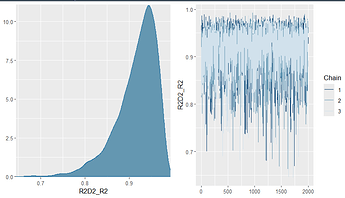
I took a look at the R2D2_R2 posteriors and made a new model with the R2D2 prior slightly closer to what I saw with R2D2(mean_R2 = 1/1.1, prec_R2 = 10) (the shiny app for R2D2 is fantastic!):

This resulted in a model with only only one prior-data conflict (on R2D2_R2) :

But when adapting the prior to make it really look like the posterior I saw R2D2(mean_R2 = 1/1.2, prec_R2 = 30):

and got a lot of prior-data conflict

(1) Am I going too far in step 2 and constraining the prior too much?
(2) Adapting the prior to the posterior seems a bit odd as I do not have a priori information on what the R2 should look like, but I guess that as long as there is no sensitivity. Is this a good way to proceed?
(3) I have played a bit more with a prior closer to the first step but I never found a settings that has no sensitivity conflict… Is it possible to widen the marginal prior distribution?
(4) Can I still go to the next step of variable selection?

---

On another note for my own understanding, I reran the model with wide student prior (student_t(3, 0, 50) in case I do not want to use R2D2 and I got plenty of weak likelihood and prior-data conflict warnings (even if the prior is really uninformative). Would the prior-data conflict comes from the fact that the prior is weakly informative in general but still more informative for some parameters than others (as covariates do not all have the same variance)? Would adapting the student prior to each parameter be the solution?

[avehtari]

@natpac

(1) Am I going too far in step 2 and constraining the prior too much?

Yes.

@natpac

(2) Adapting the prior to the posterior seems a bit odd as I do not have a priori information on what the R2 should look like, but I guess that as long as there is no sensitivity. Is this a good way to proceed?

No.

You should not simply adjust the prior until you don’t have prior sensitivity. If with your initial prior you see prior sensitivity, it means you need to think more. I’m sorry that we don’t yet have good guidance for how to think about coefficient priors for ordinal models. If you haven’t yet developed intuition about R2D2 prior, it might be better to not use it, and use something simpler for which you can more easily get understanding how to define it based on the external information. One way to gain better understanding of priors is to sample from the prior distribution and use those draws to sample from the predictive distribution, and look that the prior predictive distribution for outcomes looks reasoanble.

I also repeat that there are cases where there can be prior sensitivity on individual parameters without prior sensitivity in the quantity of interest. For example, you could examine if there is prior sensitivity for the predicted species extinction categories. It is possible that at the same time there is no prior sensitivity for predictions and there is prior sensitivity in the posterior marginals for the coefficients. This would indicate that data are not informative about the coefficients independently but do contain useful predictive information jointly. In such case you just have to accept that the data are not very informative on coefficients. You can find examples of using priorsense for predictive quantities in Bayesian data analysis - BRMS demos (@n-kall is working on making some helper functions to make it easier)

@natpac

My final aim is to use the package projpred to do some predictor selection as I expect that some factors may be redundant.

This is what you said in your first post, and even if the data are not very informative on the coefficients, you can still be possible to do variable selection in the sense of which variables are sufficient for getting similar predictive performance as the full model performance and which variables can be dropped as redundant. Nothing needs to be said about whether the variables are true or false variables. Also the causal assumptions have to come from somewhere else.

@natpac

(4) Can I still go to the next step of variable selection?

Do you have strong prior-data conflict for the predictions? Do you care only about the predictions and which variables are needed for good predictive performance, or are you going to posterior marginals of coefficients for something?

@natpac

Would the prior-data conflict comes from the fact that the prior is weakly informative in general but still more informative for some parameters than others (as covariates do not all have the same variance)?

It would be good to scale the covariates to have the same variance, as discussed in the paper. The paper has an example where different covariate scales cause prior-data conflict.

[natpac]

Thanks for the information avehtari. I think I better understand the

@avehtari

If you haven’t yet developed intuition about R2D2 prior, it might be better to not use it, and use something simpler for which you can more easily get understanding how to define it based on the external information.

I guess I have to revert back to more ‘classic’ priors for now and wait for more papers and guidance on how to use R2D2 priors… I am looking forward to it and thank you for the help still!

---

@avehtari

This is what you said in your first post, and even if the data are not very informative on the coefficients, you can still be possible to do variable selection in the sense of which variables are sufficient for getting similar predictive performance as the full model performance and which variables can be dropped as redundant. Nothing needs to be said about whether the variables are true or false variables. Also the causal assumptions have to come from somewhere else.

@avehtari

Do you have strong prior-data conflict for the predictions? Do you care only about the predictions and which variables are needed for good predictive performance, or are you going to posterior marginals of coefficients for something?

My aim is to identify the meaningful coefficients (ecological traits) that predict (/drive) the extinction risk of species (my response variable).
(1) I get that projpred can help find a simpler model with similar predictive performance as the full model, but can it indicates which variables are dropped because they do not explain much vs which are redundant ? I am asking this as I have multiple covariates and some are numeric and others are categorical so it is hard to synthetize the redundancy between them.

@avehtari

It would be good to scale the covariates to have the same variance, as discussed in the paper. The paper has an example where different covariate scales cause prior-data conflict.

(2) About scaling covariates, I already scaled the two numeric covariates (one sd, not two) but I am stuck on the categorical covariates (and ordered; they can have up to 5 levels).
I have explored the non-linear syntax but setting the global intercept to 0 does not work with ordinal model.
I saw this post on dummy/index coding but the model takes forever to run with no good convergence + I am not sure if this techniques work when having multiple categorical covariates. Do you have suggestions ?

[avehtari]

@natpac

My aim is to identify the meaningful coefficients (ecological traits) that predict (/drive) the extinction risk of species (my response variable).
(1) I get that projpred can help find a simpler model with similar predictive performance as the full model, but can it indicates which variables are dropped because they do not explain much vs which are redundant ?

Given the variables projpred selected, the non-selected variables are either irrelevant or redundant and adding them don’t improve the predictive performance.

Our paper Using reference models in variable selection discusses also the task of finding all variables that have some predictive capability alone.

@natpac

I am asking this as I have multiple covariates and some are numeric and others are categorical so it is hard to synthetize the redundancy between them.

I don’t see why. In projpred, when you add a variable either a) the predictive performance increases which indicates the variable has some predictively useful information that the already selected did not have and thus it is not redundant, or b) the predictive performance doesn’t increase which indicates the variable is either irrelevant or redundant given the already selected variables.

@natpac

(2) About scaling covariates, I already scaled the two numeric covariates (one sd, not two) but I am stuck on the categorical covariates (and ordered; they can have up to 5 levels).

Small differences in scaling is not an issue, and if you scaled the numeric covariates, things are quite good.

@natpac

I saw this post on dummy/index coding but the model takes forever to run with no good convergence + I am not sure if this techniques work when having multiple categorical covariates.

Should work. You dummy code each categorical covariate separately and put them all in the same design matrix. Not certain whether it makes thing any easier with projpred.

Are you allowed to share your data?

[natpac]

Yes, I can share the data and some basic code where prior-data conflict is limited to two coefficients. However, I’ve not managed to make it converge for now (44000 iter, 20000 warmup, 6 thin) and max_treedepth should be increased.
df_extinction.Rdata (2.0 KB)
script_STAN_ex240328.R (1.4 KB)

---

@avehtari

You dummy code each categorical covariate separately and put them all in the same design matrix.

I have done it with only 3 categorical covariate and kept one numeric and one ordered covariate but the model is not converging and takes a lot of time:

formula = extinction_cat ~ 
  + mo(cov_ordinal1)
  + cov_numeric1
  + cov_nominal1A
  + cov_nominal1B
  + cov_nominal1C
  + cov_nominal1D
  + cov_nominal1E
  + cov_nominal1F
  + cov_nominal21
  + cov_nominal3B
  + cov_nominal3C
  + cov_nominal3D
  + cov_nominal3E

[n-kall]

Thanks for providing the code and data. I experimented with the model and here are some thoughts:

1. The convergence issues seem to be due to using flat improper priors (brms default) for the regression coefficients. Changing these to e.g. normal(0, 1) or r2d2() leads to better convergence based on \hat{R}.

2. Based on loo-cv model comparison between an intercept only model and the full model (with proper priors), there is some predictive power of the full model, but it is not substantially different from the intercept model. The effective number of parameters (p_loo) for the full model is much lower than the total number of parameters in the model. This can be checked with loo and loo_compare.

3. The prior sensitivity observed in e.g. the cov_nominal3 coefficients seems to be due to weak likelihood. The posterior variance is influenced the prior, and power-scaling the likelihood has little effect on the posterior variance. This can be seen in the powerscale_plot_quantities plot of the posterior standard deviation. We are working on adjustments to the diagnostic messages provided by priorsense to make it clearer when weak likelihood is likely the cause of prior sensitivity.

4. Weak likelihood can also be shown by refitting the model with wider priors and seeing how the posterior variance increases. This may be related to having few or no observations in some of the categories (for both the outcome and the predictors). This can be further checked with the table function providing the outcome and predictor columns as arguments.

5. Unfortunately, while projpred does support cumulative family models, it does not currently support the mo() operator, so it is not currently possible to use your model with projpred without adjustment.

[harrelfe]

On a slightly related topic I’ve done some more examples where I compare Dirichlet priors on the multinomial probabilities that induce the ordinal model intercepts, vs. wide t-distribution directly for the intercepts. The Dirichlet priors always beat t priors in terms of posterior modes of intercepts and \beta agreeing with maximum likelihood estimates when there are no priors on \beta. The R rmsb package implements both Dirichlet and t priors for intercepts, for the proportional odds model.

[natpac]

Thank you n-kall for the feedback, that’s very useful. So taken with avehtari posts, it seems that the model has some weak information from the data for some coefficients but that the overall predictive power is correct (pp_check looks fine).
Given this and the high sensitivity of some coefficients to priors (leading to wider posteriors, and also slightly shifting the mean), can I still interpret all coefficient parameters with normal(0, 1) for all b_? Should I disregard or even discard the variables that have highly sensitive levels? I am concerned about the justification of the choice of the prior, normal(0, 1) is meaningful but normal(0, 2) or normal(0, 3) could be valid too.

---

On the predictors selection using projpred, I ran cv_varsel(mod, method='forward', cv_method='LOO', validate_search=TRUE, latent = TRUE, search_terms = search_terms_forced), forcing a random effect I just added on the family of the species 1|family and using the model with no monotonic effect.
plot(fitg_cv_varsel, stats = "elpd", deltas = TRUE) gives :

Predictor 1 is the forced random effect, and I see that including only 1 other predictor is enough. But the plot also seems to show that 6 predictors (including the forced random effect) could be the best.
Would keeping 6 predictors and adding back the monotonic effects make sense?

---

Just out of curiosity, do you plan to integrate monotonic effect in the projpred package soon? Thanks again for this package!

[avehtari]

@natpac

Given this and the high sensitivity of some coefficients to priors (leading to wider posteriors, and also slightly shifting the mean), can I still interpret all coefficient parameters with normal(0, 1) for all b_?

You can interpret the coefficient posteriors, but the interpretation is sensitive to the prior and collinearity. Predictive performance is probably less sensitive.

[quote=“natpac, post:19, topic:34532”]
Should I disregard or even discard the variables that have highly sensitive levels? [/quote]

If you care about the predictive performance, then no. If you care about uncertainty quantification the no, too, as discarding them corresponds to fixing them to 0 with no uncertainty. I know, statistical inference is not easy.

@natpac

I am concerned about the justification of the choice of the prior, normal(0, 1) is meaningful but normal(0, 2) or normal(0, 3) could be valid too.

If you think they are all valid, then you can report the results with all of them as prior sensitivity analysis.

@natpac

On the predictors selection using projpred

Which model did you use as the reference model? The predictive performance estimates going above the reference model result indicates the reference model might be overitting,

@natpac

Predictor 1 is the forced random effect, and I see that including only 1 other predictor is enough.

That jump is big enough that this is likely to be true.

@natpac

But the plot also seems to show that 6 predictors (including the forced random effect) could be the best.

Might be due to overfitting of the reference model or by chance due to small data set (especially for some levels)

@natpac

Would keeping 6 predictors and adding back the monotonic effects make sense?

Probably that 1 predictor is enough, unless you get better results by improving the reference model.

@natpac

Just out of curiosity, do you plan to integrate monotonic effect in the projpred package soon?

At the moment, we don’t have anyone actively adding new features (Frank Weber did a lot of work for a few years, but had to move to another job). You can create an issue in the repo, so we don’t forget this.