Gaussian distribution for logit-transformed binomial response to add an auto-regressive structure

[Lalochezia]

• Operating System: iOS 10.13.5
• brms Version: 2.6.0

TL;DR
I have a binomial response variable that is a function of five continuous covariates, but I need to account for temporal autocorrelation with an auto-regressive structure. The only way to do that is by first taking the binomial response variable, set it as a number and logit-transform it, fit the model with a Gaussian distribution, and then add the auto-regressive structure (cor_ar). This paper did the same thing with the lme{nlme} function, but there are mixed opinions about doing that kind of transformation. Such a thing can be done with brms (see below for reproducible example), but I was wondering whether it’s the right thing to do and what the opinions are with doing such a transformation (again, see below, along with other queries about weights).

The data set I’m working on is only slightly different from this reproducible example. Let’s say we have a dataset with a binomial response variable, a continuous covariate, and a sequential time covariate.

library(brms)
library(lubridate)
library(car)
library(bayesplot)

####Simulate data
#Set the seed
RNGkind('Mersenne-Twister')
set.seed(42)

#Create covariate x
x <- rnorm(1000)

#Create coefficients
beta0 <- 0.6
beta1 <- 0.7

#Create responses
z <- beta0 + beta1*x
pr <- 1/(1+exp(-z))
y <- rbinom(1000, 1, pr)

#Create timestamps
time <- seq(dmy_hms("01-01-2019 00:00:00"), dmy_hms("01-03-2019 00:00:00"), length.out = 1000)

#Create the data frame
data <- data.frame(y, x, time)
data$y <- factor(data$y, levels = c('0', '1'))

In such a case, you would fit a bernoulli or binomial distribution in a brm model:

#Control model
ctrl.mod <- brm(y ~ x, family = bernoulli(link = 'logit'), data = data, 
                seed = 42, iter = 10000, warmup = 1000, chain = 4, cores = 4)

But given the different frequency of the binomial response variable…

table(y)
y
  0   1 
393 607 

…we might want to add weights to our model.

#Weighted model
data$weights <-  ifelse(y == 1, 1, 1/(table(y)[1]/table(y)[2]))
wt.mod <- brm(y | weights(weights) ~ x, family = bernoulli(link = 'logit'), data = data, 
              seed = 42, iter = 10000, warmup = 1000, chain = 4, cores = 4)

But we have a time covariate, and we may want to account for temporal autocorrelation with an auto-regressive structure using the cor_ar function. The trouble is that it is only available for the Gaussian distribution.

This paper also sought to do the same thing. To quote from the article:

We logit transformed daily residence probabilities (adding 0.001 to 0 values and subtracting 0.001 from values of 1) and used linear mixed-effects models in the R package ‘nlme’ (Pinheiro et al. 2015), including shark ID as a random effect, and environmental covariates as fixed effects.

So I’ll try and do the same here.

#Unweighted first order AR model
data$logit.res <- logit(ifelse(y == 1, y - 0.01, y + 0.01))
ar.unwt.mod <- brm(logit.res ~ x, family = gaussian(link = 'identity'), data = data, 
                   seed = 42, iter = 10000, warmup = 1000, chain = 4, cores = 4,
                   autocor = cor_ar(~ time, p = 1, cov = F))

But we’ll create another model with an auto-regressive structure with weights for good measure:

#Weighted first order AR model
ar.wt.mod <- brm(logit.res | weights(weights) ~ x, family = gaussian(link = 'identity'), data = data, 
                 seed = 42, iter = 10000, warmup = 1000, chain = 4, cores = 4,
                 autocor = cor_ar(~ time, p = 1, cov = F))

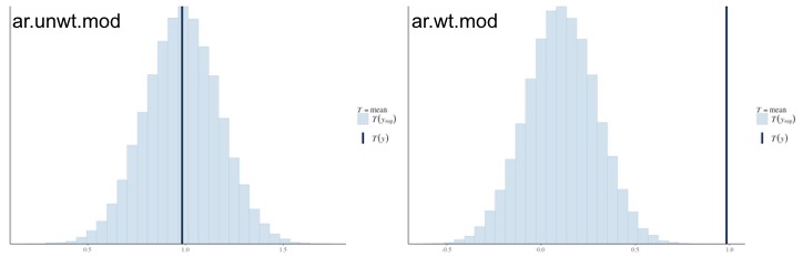
The coefficients aren’t so important. What I’m most concerned about are the posterior predictive distributions:

The models on the left are unweighted models, those on the right are weighted. Top row is fitted with a Binomial distribution, bottom row is fitted with a Gaussian distribution with a logit-transformed response variable.

The ctrl.mod has a good fit, but when we include weights, the wt.mod doesn’t fit very well because of the weights. What’s really concerning are the bottom two graphs. In order to fit an auto-regressive structure to account for temporal autocorrelation, I had to logit-transform the response variable and fit a Guassian distribution, which is reflected in the posterior predictive distribution. But because I fitted the auto-regressive structure, the fit really suffers; the mean of the posterior distribution is hanging in between the two observed values found in the data, differing due to the weights (or lack-thereof) of the response variable.

The LOO-PIT plots are pretty wild as well:

Same as previous figure

What’s happening in the top two graphs is beyond me. The bottom graphs look typical of a non-normal distribution, which make sense since the data isn’t normally distributed anyway.

Mean recoveries are also varied (I could only get mean recoveries for the AR models, the two binomial models kept returning polygon edge not found as an error):

The unweighted AR model had decent mean recovery, but the weighted AR model was way off.

This answer to this question said that logit-transforming the response variable is not advised, though a comment to the answer said that this type of transformation is very common (such as the previously linked paper). Hence why I thought it’d be all right to do this with brms, especially since I need to account for temporal autocorrelation. But then again, I’m not sure.

Although this is a simulated dataset, the bayesplot presented here exactly the same plots I’m getting for my dataset.

My questions are:

1. Is it more important to ensure the posterior predictive distributions fit the observed distribution of the data?
2. Should weights be used at all if it means the distributions will not align or if mean recoveries are way off? Are imbalances in the response variable generally handled differently within a Bayesian framework? Because it seems adding weights is getting some poor fits all around, so I’m wondering if I should do away with them entirely.
3. When we need to account for temporal autocorrelation, is logit-transforming the binomial response variable and specifying a Gaussian distribution the best way to go just so that we can fit an autoregressive structure, even if the distributions don’t align? If not, what’s the best way to account for temporal autocorrelation with a binomial response variable?

[paul.buerkner]

As of brms 2.9.0, you should be able to use the cor_ar correlation structure with binomial responses. You may need to set cor_ar(..., cov = TRUE) though.

[Lalochezia]

Thanks @paul.buerkner, I’ll go ahead and update it now. Should I keep using weights, though? In the example I provided here, there wasn’t much of an imbalance, but my data set had a 1:14 ratio in the response variables, so I thought I should probably keep them.

[paul.buerkner]

If you include all your single responses in your data frame that why would you want to weight them additionally?

[Lalochezia]

Not sure, to be honest. I was always under the impression that heavily unbalanced data always needed weights, but didn’t know that if I include all my single responses in the data frame that I wouldn’t need any weights at all.

[paul.buerkner]

I did not look into your example in detail, but if you include all single responses, is any of them worth more than others? Asked differently, what’s the purpose of the weights in this context?

[Lalochezia]

No, none of the levels in the response variable is worth more than others. The weights were just added so that the lower frequency of one response variable would be ‘equal’ to that of the more frequent response variable. It was something I had to do with a decision tree analysis since I had a lot more zeros than ones and the decision tree at the time wasn’t handling the imbalance very well.

[paul.buerkner]

Not sure if that’s a statistically sound approach, though, it may be in some fields and it certainly depends on your target of inference. Anyway, at least you can try to model autocorrelation now. Be aware though that autocorrelations require latent residuals (which are automatically added by cor_ar), which may not be identified for a binary response. So you may very well run into additional problems.

[Lalochezia]

If you don’t think it’s statistically sound, then I probably won’t go ahead and do it. I don’t have as much experience as I would like so any advice from someone who understands this better than me is probably worth heeding.

Could you elaborate on the latent residuals bit? What are they, and why would it not be identified in a binary response?

[Max_Mantei]

First, as I see it, weighting is usually not the elegant solution, as it “artificially” downplays information that you have got. I’ve seen corrections being used for highly imbalanced logit models in frequentist context, but that usually means a class balance of 9:1 or higher. As I understand, frequentist methods are all about the sampling distribution and you generalize your inference from that, while Bayesians stick to the posterior distribution - and it seems that that looks very reasonable in your case (without weighting). This is the second thought I had: I’d hardly call a 2:3 ratio imbalanced.

If you are doing weighting because of another methods you used before, I wouldn’t stick with it. In any case, you could still post-stratify the posterior to match the population you want to generalize to.

[Lalochezia]

Thanks @Max_Mantei. The example I had here has a 2:3 ratio imbalance, but my actual dataset is much higher than 1:9, more around 1:14-15 range. That said, if Bayesians stick to posterior distributions, then should I not weight my response variables anyway?

[Max_Mantei]

Check this discussion about weighting.

Also, afaik weighting is used to make the sample that you have resemble the population you want to generalize to (in frequentist statistics!). This is why y_rep in the wt.mod model shows you that both classes are equally likely in the posterior… You basically told the model, that the 2:3 ratio in the data is really a 1:1 ratio in the population.

In a Bayesian model, the more natural way to give the model this information is the prior! If you have strong prior belief, that the population ratio of ones and zeroes is 1:1, then you’d but a very strong prior on the intercept term centered at zero (assuming, that all covariates are centered).

The same logic follows if your data is 2:3, but you’d expect a 1:14 (sorry that I didn’t read that before, I should have read the thread more carefully!) ratio in the population. A frequentist would weight the data, so it matches the population ratio. As a Bayesian, you’d just put your prior information into the model.

Now, all of this is really not that important if a) the sample ratio of ones and zeroes matches that of the population, and b) when you are only interested in the slopes (coefficients) of the covariates (which should still be “consistent estimators”).

---

And, as an aside (I think you are probably aware of this), working with something like this:

logit(ifelse(y == 1, y - 0.01, y + 0.01))

is really bad if y \in \{0,1\} as in your generated data (i.e. y can only be 0 or 1). In the bit, that you quote, it seems Pinheiro et al. have y \in [0,1], i.e. y can be 0 or 1 or anything in between.

[Lalochezia]

Thanks for the thorough response, @Max_Mantei. I’m new to Bayesianist philosophies and I’m finding it hard to not apply frequenist principles, so I think I have fair amount of work left to do.

I’m at my wit’s end with the data I’m trying to analyze, is it all right if we can take our chat outside of the forum? If there’s anyway I could message you (I don’t think I have those privileges yet though…).

[Max_Mantei]

No worries. You might want to check out @richard_mcelreath’s lectures. I think he is doing a great job explaining the Bayesian approach “from scratch” and has nice visualizations and interesting examples. Only heard good things about his book (maybe one bad thing is the price…).

Honestly, I’m not sure, if I can help you with the details of your model - I don’t know that much about AR(1) processes for binary outcomes. In any way I think it is preferably to have these discussions in public, because users with similar problems might benefit from reading the thread - that is, if you are allowed to make these parts of your project public.

All that being said, I’d give the latent variable probit model, that is described in the Stan user guide a chance. Set it up and add the lagged latent utility as predictor variable. If you think stationarity is ensured, you can constrain its coefficient to [-1,1]. There’s also a fair bit on AR stuff in the manual.

[Max_Mantei]

Hm, one more thought: Does something like this

mod <- brm(y ~ x + s(time), family = bernoulli(link = 'logit'), data = data)
(where you have time as sensibly chosen numeric variable)

yield reasonable results for your real/original data?

[Lalochezia]

Hi @Max_Mantei, sorry for the delay in replying! I haven’t given that (or the other one you recommended) a try yet, it’s been busy at work but I’m going to let this monster run over the long weekend and see where it gets us. I’ll let you know what happens once the results come in!

[Lalochezia]

At the moment the bernoulli model with a smoother on the time variable is running. I haven’t started reading the Stan User Manual yet, though I’ve downloaded the book and will make it my light weekend reading (on top off a copy of Statistical Rethinking).

I’m going to make the data set available here if you want to give it a try. Once the model is done, I’ll fit the probit model and see where that leads me.

data1.csv (606.2 KB): var1:var5 are scaled
data2.csv (577.9 KB): var1:var5 are unscaled and in their original units.

The other thing I’m not sure about is how to add the lagged latent utility as a predictor variable. Is that the me() function?

I’ve also attempted to run a binomial model with the cor_ar() function with cov set to TRUE, but it was taking too long (1800 seconds for 1000 transitions using 10 leapfrog steps per iteration).

[Max_Mantei]

This is my approach after thinking about it and remembering that @jonah had something really clever in his pest control example in the tutorial in StanCon Helsinki (2018).

One problem might be that the time intervals are not evenly spaced. I’m not sure, but I think a continuous AR(1) process is actually a Ornstein-Uhlenbeck process. Also, you might want to check out the R ctsem by @Charles_Driver. I’ve never used it before, but I guess it’s exactly for stuff like this.

Anyways, this code runs the model for one of the ID (in this example ID == 3). You would have to extend it to more groups. Also, this code runs the AR(1) prior on the specific time points – since these are unevenly spaced, I also included two lines, which let’s you run the AR(1) process to model the correlation between days (it also models missing days automatically)…

library(tidyverse)
library(readr)
library(rstan)
options(mc.cores = parallel::detectCores())
rstan_options(auto_write = TRUE)

data <- read_csv("data1.csv", 
                 col_types = cols(X1 = col_skip())) %>% 
  arrange(utc) %>% 
  filter(ID == 3) %>% 
  mutate(#day = lubridate::floor_date(utc, unit = "day"), # un-comment if AR(1) by days
         #time = as.numeric(difftime(day, min(day), units = "days")) + 1) # un-comment if AR(1) by days
         time = 1:n()) # comment out if AR(1) by days

stan_data <- list()
stan_data <- within(stan_data,{
  N <- nrow(data)
  X <- model.matrix(~ 0 + var1 + var2 + var3 + var4 + var5, data = data)
  K <- ncol(X)
  t <- max(data$time)
  y <- data$y
  time_idx <- data$time
})

posterior <- stan(file = "stan_model.stan", data = stan_data)
print(posterior)

Where stan_model.stan is:

data{
  int<lower=0> N;
  int<lower=0> K;
  int y[N];
  matrix[N,K] X;
  int t;
  int<lower=1,upper=t> time_idx[N];
}
transformed data{
  matrix[N,K] Q = qr_thin_Q(X)*sqrt(N);
  matrix[K,K] R_inv = inverse(qr_thin_R(X)/sqrt(N));
}
parameters{
  real alpha;
  vector[K] beta_tilde;
  real<lower=0> sigma_time;
  real<lower=0,upper=1> rho_raw;
  vector[t] time_raw;
}
transformed parameters{
  vector[N] mu = alpha + Q*beta_tilde;

  // AR(1) process priors
  // (inspired by Jonah Gabry's Helsinki Stan tutorial)
  real rho = 2.0 * rho_raw - 1.0;
  vector[t] time = sigma_time * time_raw;
  time[1] /= sqrt(1 - rho^2);
  for (i in 2:t) {
    time[i] += rho * time[i-1];
  }
  
  mu += time[time_idx];
}
model{
    
  y ~ bernoulli_logit(mu);

  alpha ~ normal(-5, 5);
  beta_tilde ~ normal(0, 2.5);
  rho_raw ~ beta(10, 5);
  time_raw ~ std_normal();
  sigma_time ~ std_normal();

}
generated quantities{
  vector[K] beta = R_inv*beta_tilde;
}

---

Model for time points:
First is just the time variable from the model code, second is inv_logit(mu).

---

Model for days:
First is just the time variable from the model code, second is inv_logit(mu).

If all of this makes sense, I don’t know. But maybe this’ll give you a place to start.