Hello. I’m playing with brms trying to fit a multilevel model to rheological data, and I’m getting results for model prediction with no physical meaning. I’m here trying to get help in how to set up my model to avoid this problem. My background in statistics is lackluster, so pardon me if I make some mistake while writing this post.
Background: I have a very large database of lab measurements of the flow behaviour of a clay suspension, which behaves as a non newtonian fluid. Using a rotational rheometer, we force the sample through different shear rates, and record the applied shear stress on the fluid, through 4 different loading “phases”. We hypothesize that the fluid behaviour is dependant on the solids content of the sample and on the the test “phase”. The acquired database is as follows:
> head(dat_teste)
  sample   phase  SC   gamma   tau
1 A020102      2  60  70.030  3164
2 A020102      2  60  38.490  2810
3 A020102      2  60  20.480  2522
4 A020102      2  60  10.880  2292
5 A020102      2  60   5.796  2148
6 A020102      2  60   3.085  2028
In which ‘phase’ is the test phase (numeric, integer, categorized), ‘SC’ is the solids content (numeric, integer, categorized), ‘gamma’ is the recorded shear rate (numeric), and ‘tau’ is the recorded shear stress (numeric). There are two different values for ‘phase’ and three different values for ‘SC’ in the small part of the database I’m using as test.
The data, for a given sample, should follow the Herschel-Bulkley model:
\tau=a+b \gamma ^c
With a, b and c as the model parameters.
Model construction in brms: I’m following Granville Matheson’s brms nonlinear modelling syntax guide, which I could adapt with relative success. I set up my model as follows:
model_HB <- brms::bf(tau ~ a + b * (gamma^c),
                     a ~ 1 + (1|SC) + (1|SC:phase),
                     b ~ 1 + (1|SC) + (1|SC:phase),
                     c ~ 1 + (1|SC) + (1|SC:phase),
                     nl = TRUE)

prior <- c(prior(uniform(10, 5000), nlpar = 'a', lb = 10, ub = 5000),
           prior(uniform(1, 1000), nlpar = 'b', lb = 1, ub = 1000),
           prior(uniform(10^-3, 1), nlpar = 'c', lb = 10^-3, ub = 1))

fit1 <- brm(formula = model_HB ,
             data = dat_test,
             family = brmsfamily('Gaussian'),
             prior = prior,
             control = list(adapt_delta = 0.9),
             iter = 10000,
             warmup = 5000,
             thin = 5,
             chains = 4,
             seed = 123)
The fit appears to have run with no problems.
> summary(fit2)
Group-Level Effects:
~SC (Number of levels: 3)
                Estimate Est.Error l-95% CI u-95% CI Rhat Bulk_ESS Tail_ESS
sd(a_Intercept)   643.46    337.97   228.17  1523.17 1.00     3726     3434
sd(b_Intercept)    63.67     79.45     1.70   292.74 1.00     3619     3865
sd(c_Intercept)     0.23      0.29     0.01     1.01 1.00     3527     3937

~SC:phase (Number of levels: 6)
                Estimate Est.Error l-95% CI u-95% CI Rhat Bulk_ESS Tail_ESS
sd(a_Intercept)   146.06    125.44    29.41   503.74 1.00     3520     3360
sd(b_Intercept)    35.06     31.49     1.80   118.06 1.00     3637     3643
sd(c_Intercept)     0.07      0.08     0.00     0.28 1.00     3713     3703

Population-Level Effects:
            Estimate Est.Error l-95% CI u-95% CI Rhat Bulk_ESS Tail_ESS
a_Intercept   872.30    378.63   188.42  1719.29 1.00     3640     3363
b_Intercept    92.10     50.44    17.71   222.20 1.00     3623     3702
c_Intercept     0.49      0.15     0.15     0.82 1.00     3952     3774

Family Specific Parameters:
      Estimate Est.Error l-95% CI u-95% CI Rhat Bulk_ESS Tail_ESS
sigma   557.86      7.16   543.97   572.04 1.00     4081     3929
However, when investigating results, I came across this problem: when computing intervals from the posterior predictive distribution, I get negative values for ‘tau’, which have no physical meaning in this case.
> predictive_interval(fit2)
                   5%      95%
...
 [123,]  269.22861269 2101.801
 [124,]  164.59882127 1972.046
 [125,]   68.15528121 1889.180
 [126,]    7.18404354 1826.386
 [127,]  -45.07619383 1788.156
 [128,]  -76.17254151 1747.468
 [129,] -104.48853666 1745.090
 [130,] -121.93558750 1728.839
 [131,] -149.53286987 1693.427
 [132,] -120.25919652 1664.096
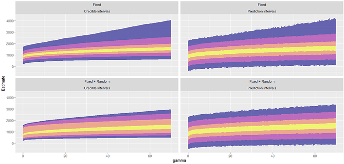
Following Matheson’s guide, I plotted this graph, which also shows this problem for the prediction intervals (obtained using the predict() function). Credible intervals (obtained using the fitted() function) seem fine.
Can anyone please help me in figuring out how to fix this?
Any help is deeply appreciated.
- R version 4.3.1
- brms version 2.20.4

