Double-Pareto Lognormal Distribution in Stan

Hi everyone,

I made an attempt to code up the Double Pareto LogNormal Distribution in Stan. The attached R file shows DPLN data generation using equation 6 of Reed and Jorgensen (https://www.math.uvic.ca/faculty/reed/dPlN.3.pdf) and the file DPLN-fit.stan fits the model using the pdf in the form of equations 8 and 9 (noting the typo in Eq 9, where alpha should be theta). I wrote two different version of the function, one which takes in scalars and one for vectors (I comment out the one I don’t want as I go), but the guts are the same.

The model with the vector version of the function is:

functions {
real dpln_log(vector x, real alpha, real beta, real nu, real tau){
  vector[num_elements(x)] prob;
  real lprob;
  real leadfraction;
  leadfraction <- (alpha*beta)/(alpha + beta);
  for(i in 1:num_elements(x)){
    prob[i] <- leadfraction*(  exp(alpha*nu + 0.5*square(alpha*tau))*pow(x[i],(-alpha-1))*Phi(inv(tau)*(log(x[i]) - nu - alpha*square(tau)))      +      exp(-beta*nu + 0.5*square(beta*tau))*pow(x[i],(beta-1))*(1 - Phi(inv(tau)*(log(x[i]) - nu + beta*square(tau))))   );
    }
  lprob <- sum(log(prob));
  return lprob;
  }
}
data {
  int N;
  vector[N] x;
}
parameters {
  real<lower=0> alpha;
  real<lower=0> beta;
  real nu;
  real<lower=0> tau;

}
model {

  // priors
  alpha ~ cauchy(0,5);
  beta  ~ cauchy(0,5);
  nu ~ normal(0,50);
  tau  ~ cauchy(0,5);

  // likelihood
  x ~ dpln(alpha, beta, nu, tau);

}

The sampling behaviour is very unhealthy and the inference is mediocre (although actually sometimes ok, and usually in fact not as bad as it should be given how bad the sampling is!). The attached traceplots show something weird: some of the chains look ok but some are essentially degenerate / perfectly autocorrelated. I haven’t see this happen before. Is anyone familiar with these patterns, or alternatively, with these kinds of composite distributions?

As you can see, the number of effective draws is laughable in this case, but I noticed it’s also quite variable across runs:

I may have made a typo in the definition of the function – but the presence of the good chains makes me think it’s not that. Also, I did check that my function can be used to generate data that looks approximately right to me when I switch the parameters / data blocks around (see second part of the attached R file and the DPLN-generate.stan files – yes I did it in the model block, I see this as a check not a serious data generation attempt, and I include it just in the interest of completeness).

The DPLN might just be a badly-behaved distribution, and certainly it only has moments smaller than the alpha parameter, but I have tried with larger values of alpha (eg 10) and did not see much improvement.

I wondered if the half-cauchy priors are just too wide for this relatively complex distribution, and I tried once with tighter!half-normal priors – that actually made it worse, all the chains were badly autocorrelated. Curious!

Any insight much appreciated! Hopefully once we get to the bottom of this all stan users will be able to enjoy the DPLN. :)

Cheers
Rachael

DPLN-fit.stan (1.3 KB)
DPLN-generate.stan (1.2 KB)
DPLN-test.R (2.2 KB)

1 Like

See Section “Testing the user defined functions” in Extreme value analysis and user defined probability functions in Stan for instructions how test user defined distribution functions.

I also suggest plotting the distribution with parameter values from the stuck chain and compare to your data. It’s possible that there is a narrow mode in the posterior near these values.

1 Like

I think equation 28 in the paper may have been a better choice, but if I were to implement equations 8 and 9, I would have done it like
EDIT: This was completely wrong.

functions {
  real dpln_lpdf(vector x, real alpha, real beta, real nu, real tau) {
    int N = rows(x);
    real log_leadfraction = log(alpha * beta) - log(alpha + beta);
    real tau2 = square(tau);
    real tau_inv = inv(tau);
    real log_A1 = alpha * nu + 0.5 * square(alpha) * tau2;
    real log_A2 = -beta * nu + 0.5 * square(beta)  * tau2;
    real coef1 = beta - alpha - 2;
    real coef2 = alpha * tau2;
    real coef3 = beta  * tau2;
    real log_kernel = 0;
    for (n in 1:N) {
      real log_x = log(x[n]);
      real log_xmnu = log_x - nu;
      log_kernel += coef1 * log_x + log(Phi(tau_inv * (log_xmnu - coef2))) + 
                                  log1m(Phi(tau_inv * (log_xmnu + coef3)));
    }
    return log_kernel + N * (log_leadfraction + log_A1 + log_A2);    
  }
}

This version does all of the calculations in terms of log units in order to maximize numerical stability and reduces the amount of autodiff by adding N times the sum of the constants to the accumulated log kernel (if seen as a function of x).

1 Like

Thank you Aki and Ben!

Aki: that reference is super useful and so is the suggestion to check for local modes, I’ll do that and report back.

Ben: I implemented the version of the function you wrote and it samples extremely well and recovers nu and tau excellently, but it can’t recover alpha and beta at all. I think there must be a typo somewhere (relatedly, I can’t quite see how you managed to get from the log of the sum in equation 8 of the paper to the sum of the logs in your function here) but I haven’t managed to fix it yet. I’m working on that now and will update when I have a solution, which may involve following your hunch and just coding up equation 28 instead, let’s see.

The trick is to misread the paper as saying everything gets multiplied. Alternatively, you could use log_sum_exp as in

functions {
  real dpln_lpdf(vector x, real alpha, real beta, real nu, real tau) {
    int N = rows(x);
    real log_leadfraction = log(alpha * beta) - log(alpha + beta);
    real tau2 = square(tau);
    real tau_inv = inv(tau);
    real log_A1 = alpha * nu + 0.5 * square(alpha) * tau2;
    real log_A2 = -beta * nu + 0.5 * square(beta)  * tau2;
    real coef1 = -alpha - 1;
    real coef2 = alpha * tau2;
    real coef3 = beta - 1;
    real coef4 = beta  * tau2;
    real log_kernel = 0;
    for (n in 1:N) {
      real log_x = log(x[n]);
      real log_xmnu = log_x - nu;
      log_kernel += 
        log_sum_exp(log_A1 + coef1 * log_x + log(  Phi(tau_inv * (log_xmnu - coef2))),
                    log_A2 + coef3 * log_x + log1m(Phi(tau_inv * (log_xmnu + coef4))));
    }
    return log_kernel + N * log_leadfraction;
  }
}

but this also does not produce the right answers yet.

2 Likes

I tried to re-do this with the log likelihood from equation 28 – it also contains a typo, FYI, it should be the log of the Gaussian pdf there (assuming, as I do, that eq 28 is supposed to just be the log of eq 5).

The resulting model almost works. This is driving me nuts: 3 of the 4 chains consistently nail all the correct parameters and sample pretty well. 1 chain stuffs everything up.

Here’s the function:

functions {
  real dpln_lpdf(vector x, real alpha, real beta, real nu, real tau) {
    int N = rows(x);
    real log_leadfraction = log(alpha) + log(beta) - log(alpha + beta);
    real tau_inv = inv(tau);
    real coef1 = alpha * tau;
    real coef2 = beta  * tau;
    real log_kernel = 0;
    for (n in 1:N) {
      real log_x = log(x[n]);
      real log_xmnu_std = tau_inv*(log_x - nu);
      real p = coef1 - log_xmnu_std;
      real q = coef2 - log_xmnu_std;
      real Rp = (1-Phi(p))/exp(normal_lpdf(p|0,1));
      real Rq = (1-Phi(q))/exp(normal_lpdf(q|0,1));
      log_kernel +=   std_normal_lpdf(log_xmnu_std) + log(Rp + Rq) ;
    }
    return log_kernel + N*(log_leadfraction);
  }

(yes it is awkward that to get the normal pdf for the mills ratio I have to exponentiate the normal lpdf function… if someone knows a better way please let me know)

Here’s the output, note that the true values in this case are alpha = 2, beta = 2, nu = 5, tau = 2, so the 3 well-functioning chains are exactly right in this case:

I am now struggling to figure out what went wrong with chain 1 still and whether it’s something I can predict and prevent. Also in case this helps anyone figure it out: stan wants me to increase max treedepth and adapt delta, but actually doing either or both makes the problems worse not better.

I think you can do log_sum_exp(log_Rp, log_Rq) where the inputs are defined as

real log_Rp = log1m(Phi(p)) - std_normal_lpdf(p);
real log_Rq = log1m(Phi(q)) - std_normal_lpdf(q);

But it would be better to do the std_normal_lpdf(log_xmnu_std) outside the loop because it can accumulate the gradient over observations. So, I think it would be

  real dpln_lpdf(vector x, real alpha, real beta, real nu, real tau) {
    int N = rows(x);
    real log_leadfraction = log(alpha) + log(beta) - log(alpha + beta);
    real tau_inv = inv(tau);
    real coef1 = alpha * tau;
    real coef2 = beta  * tau;
    real log_kernel = 0;
    vector[N] log_x;
    for (n in 1:N) {
      real log_x_n = log(x[n]);
      real log_xmnu_std = tau_inv * (log_x_n - nu);
      real p = coef1 - log_xmnu_std;
      real q = coef2 - log_xmnu_std;
      real log_Rp = log1m(Phi(p)) - std_normal_lpdf(p);
      real log_Rq = log1m(Phi(q)) - std_normal_lpdf(q);
      log_kernel +=  log_sum_exp(log_Rp, log_Rq);
      log_x[n] = log_x_n;
    }
    return log_kernel + normal_lpdf(log_x | nu, tau) + N * log_leadfraction;
  }

Also, it would faster if the function’s signature were defined in terms of a vector y where y = log(x); so that you don’t have to take the logarithm of constants millions of times.

I would try making init_r smaller than its default of 2 if there is a positive probability that the adaptation fails.

3 Likes

Good points all around, thank you Ben! I implemented the above but changed everything to be in terms of y= log(x), and I also fixed a typo (it should be q = coef2 + log_xmnu_std) but alas we still have the same old sampling problems.

I have now implemented a simpler version of the model, the Pareto-Lognormal, and done it entirely on the log(x), which is to say I wrote a Normal-halfLaplace model on the variable y from Reed and Jorgenson. I wrote the lpdf function by taking the log of equation 13. This model actually works in some regions of the parameter values! But it does not work when alpha is large. And in all cases there is a persistent weirdness in stan where it reports lots of divergent transitions (even when the model is fitting great) – and as before, raising adapt_delta makes the problem much worse!

functions {
   real normalhalflaplace_lpdf(vector y, real alpha, real nu, real tau) {
    int N = rows(y);
    real log_alpha = log(alpha);
    real tau_inv = inv(tau);
    real coef1 = alpha * tau;
    vector[N] lprob;
    for(n in 1:N){
    real y_std;
    real p;
    real log_Rp;
      y_std <- tau_inv*(y[n] - nu);
      p <- coef1 - y_std;
      log_Rp <- log1m(Phi(p)) - std_normal_lpdf(p);
      lprob[n] <- std_normal_lpdf(y_std) + log_Rp;
    }

  return sum(lprob) + N*log_alpha;
  }
}
data {
  int N;
  vector[N] y;
}
parameters {
  real<lower=0> alpha;
  real nu;
  real<lower=0> tau;

}
model {

  // priors
  alpha ~ cauchy(0,10);
  nu ~ normal(0,10);
  tau  ~ cauchy(0,10);

  // likelihood
  y ~ normalhalflaplace(alpha, nu, tau);

}

(I didn’t use the log_kernel syntax purely because I’m too afraid I’ll introduce bugs due to my lack of familiarity with that structure.)

I now think this distribution actually has some problems that the authors haven’t fully copped to. Reading the section on estimation closely, I see: “Experience has shown that it is worthwhile examining the data for evidence of power-law behaviour in the tails. If for example there
is only power-law behaviour in one tail, attempts to fit the dPlN may result in
the non-convergence of the optimization algorithm”. That is to say on the full model if either beta or alpha is large, the distribution model doesn’t really work in some unspecified way. Well, by the same token, even in the simpler model here where beta is eliminated, a large alpha would imply that the whole model should actually just be Gaussian on y.

I suspect this is due to identification problems – I think the tail of a thin-tailed-Laplace is nearly or indeed completely indistinguishable from the tail of a Normal (in this paper’s notation, large alpha means a thin tail; alpha is defined as the reciprocal of sigma in the stan manual for the double exponential). By the same token, I’ve noticed that thinner-tailed Paretos can look quite similar to the tail of a very platykurtic Lognormal in practice (but I should note, serious econometricians have told me this shouldn’t be the case…).

I also noticed that the parameters of this model seem to be able to “disagree” with each other. For example, if alpha is large (thinner tails) fit gets worse as nu gets far away from zero, holding tau constant. In some sense here the two bits of the model are working against each other: nu says there should be mass far from zero, alpha says there shouldn’t be.

I hold out some hope that a fancy re-parameterisation using gaussian and exponential component draws to construct y in the model block might cure some of the divergent transitions, and I will attempt that now. [Edited to add: this was a foolish and also incoherent hope, based on the error of thinking you can reparameterise a data variable. Lol.]

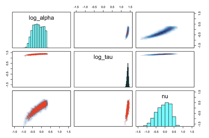
Can you share the pairs plots for log alpha, nu, and log tau? Especially an overlay of the divergent and non-divergent samples? The non-identifiability should be pretty clear there.

The next step would be looking at how the identifiably changes with parameter values, which you can study by fitting prior predictive data.

Also get rid of those Cauchy priors!

I would not at all be surprised if there are seriously identifiability problems in these models but at the same time kind of excited to see how they manifest!

1 Like

Thanks for joining Mike! Yes absolutely I can provide the pairs plots. I have also changed the priors to normal (is that what you were hoping for?) in this case it doesn’t seem to have affected the output much (which is better than before where it made things worse).

Here is the pairs plot in a case where the inference is pretty good (alpha = 2, tau = 2, nu = 1, all inside their 95% intervals and tau is in its 50% interval) but still got a lot of divergent transitions:

Now here’s a case where the laplace tail is thin and the normal is more dispersed, so the inference is bad (alpha = 10, tau = 4, nu = 1), only tau is in the 95% interval and none are in the 50% interval. But to me the pairs plots here look similar to the above. Does that imply this is not an identifiability issue? Or what do you think?

Even in the first case the model is pretty poorly identified, at least in the way we use identified. Maybe we shouldn’t use the “I” word since it has so much baggage – there’s the frequentist asymptotic definition of “does the estimator converge to a unique point that is the true value” and the more Bayesian usage of “does the posterior concentrate into a small neighborhood” which are related but not identical concepts.

In any case, one can’t really talk about the exact posterior behavior because of the divergences. In particular in the second circumstance it looks like the sampler is trying to move to larger alpha (and possibly nu) but can’t navigate the geometry (hence the divergences). To verify this you can run with adapt_delta set to a higher value, say 0.95, running again and comparing the pairs plots to what you have above. It will probably be annoying, but if you can put consistent axis limits on all of the pairs plots that would make comparisons much easier.

Also keep in mind that there’s no guarantee that the posterior will cover the true value for any given observation – the only guarantees we have are when averaging over fits from prior predictive data. So here I’m not so much looking for where the posterior is relative to the true values but rather the posterior shapes.

2 Likes

log_alpha seems to have scary quick change in the density at the right side, which can cause problems, too

Yeah, but I think that might be due to divergences. You see the same behavior in the second fit, too, even though the true log alpha is all the way at log(10) ~ 2.3 suggesting that the posterior fit is being cut off.

Ok, I set adapt_delta = .95 and made the axes limits consistent across all subpanels for the two models. This is interesting. Here’s the “good” case:


Here’s the bad case:


We do see fewer divergent transitions in the good case here especially in the panels in the top right corner. In both cases it seems that the problem is really in the lower left corner panels but I don’t really know what to conclude from this. (I had thought these plots should be mirrored on the downwards-45-degree line but I am obviously wrong about that and must have misunderstood the plots in the past.) Does anything jump out at you guys?

If these are RStan pairs plots then the red on the lower diagonal and upper diagonal mean different things. I think lower diagonal indicate divergent transitions and upper diagonal indicate transitions that saturated the max treedepth, but I could be wrong.

What you really want to compare is not these two plots to each other but rather two the previous two plots. Could you plot the log_alpha vs log_nu points for the two adapt_delta settings on top of each other (you’ll have to do this yourself, but you don’t need to plot divergences for the comparison so it should be straighforward). What you want to look for is in which direction the fit expands as you increase adapt_delta.

My hunch is that the gradients explode as alpha increases which is causing the divergences. That said, the fact that the alpha=10 fit results in a narrower posterior than the alpha=2 fit is…suspicious.

Are you running with the default four chains?

1 Like

By default, the lower panels are those with below median accept_stat__ and the above panels have above median accept_stat__.

3 Likes

yes, 4 chains. Here’s the bad case with the two different adapt_delta values (0.8 on top so we can see how it moves away from that):

Here’s the good fit case:

To me it looks like there isn’t anything much different between the two adapt delta values but perhaps this is my untrained eye?

Perfect!

No, your eye is correct here. There really isn’t a difference which means that the problem isn’t strongly geometric. That suggests that it might be more of the density implementation being unstable, or even the autodiff’d gradient being unstable which isn’t uncommon in complex models.

Can you post the data and most currently model you’re using? I’ll take a look this weekend.

2 Likes

Awesome, so glad we are making progress understanding this! Thanks for all your help so far.

Thank you also for any time you spend taking a closer look at this. The current model is a one-tailed version of the double-pareto-lognormal, so just a pareto-lognormal per equation 13 in Reed and Jorgenson. This will be all I need for my application anyway, so if we can understand this one I will be very very happy. I do it on the log scale so it’s a normal-half-laplace (or probably should be called a normal-exponential). The data is simulated per Reed and Jorgenson’s suggested method using gaussians and exponentials (but setting beta = infty, to get this subcase).

Attached files below:

normalhalflaplace-fit.stan (836 Bytes)
single-pareto-lognormal-test.R (4.2 KB)

2 Likes

I’ll go through my through process so that there’s an example of how to track down fitting problems in models you haven’t used before.

Changing adapt_delta, and hence the accuracy of the symplectic integrator used by the Hamiltonian transition, didn’t affect the posterior fit which immediately suggested to me that there was a problem of numerical accuracy in your new density function instead of any geometry problems. Numerical inaccuracies lead to inaccurate gradients which break all of the wonderful properties of symplectic integrators, regardless of the step size; seeing the pathology unchanged as adapt_delta, and hence the step size, is typically a sign of numerical problems.

Indeed inspecting your normalhalflaplace_lpdf function one sees log1m(Phi(p)) which is an immediate red flag. For | p | \gtrapprox 5 the Phi function starts to saturate near 0 or 1 and loses precision which then causes the log1m evaluation to be significantly inaccurate. The resulting gradient is even worse. See https://github.com/stan-dev/math/issues/1284 for some recent discussion.

With that suspicion in mind I ran your code with data simulated from \alpha = 10 but printed out the (\alpha, \nu, \tau) configuration whenever | p | > 6. Every instance occurred for \alpha and \nu at their largest values, where you saw cutoffs in your posterior fits. In other words your posterior fit couldn’t go past those boundaries you saw because your log density function implementation wasn’t sufficiently accurate.

Then I went I a little bit too far and played around with asymptotic series to implement a more accurate log density function for p > 6. This ended up giving

real normalhalflaplace_lpdf(vector y, real alpha, real nu, real tau) {
  int N = rows(y);
  vector[N] lpd;
  for(n in 1:N) {
    real y_std = inv(tau) * (y[n] - nu);
    real p = alpha * tau - y_std;
    real log_Rp = 0;
    
    if (p > 6) {
      real inv_p = inv(p);
      real inv_p_sq = square(inv_p);
      real variable = 1;
      real coefficient[7] = {-1, 2.5, -12.3333, 88.25, -816.2, 9200.83, -122028};
      
      log_Rp = log(inv_p);
      for (i in 1:7) {
        variable *= inv_p_sq;
        log_Rp += coefficient[i] * variable;
      }
    } else {
      log_Rp = log1m(Phi(p)) - std_normal_lpdf(p);
    }
    
    lpd[n] = std_normal_lpdf(y_std) + log_Rp;
  }
  return sum(lpd) + N * log(alpha);
}

Running with this still gives a few divergences, but this time for small \alpha. The posterior, however, captures the simulated ground truth of \log(10) ~ 2.3.

The divergences for small \alpha could be due to numerical inaccuracies for p \lessapprox -5, but the pinching/funnel like shape suggests that it might also be inherent to the geometry of your problem and resolvable with a higher adapt_delta (the above plot was with default values). I also tried an asymptotic expansion for \log(1 - \Phi(x)) around x = \infty to account for possible numerical problems but couldn’t get anything to work.

Long story short: you were having fitting problems because of numerical instabilities in \log(1 - \Phi(x)) for x \gtrapprox 6. Adding a more robust implementation recovers a much better fit. That fit, however, demonstrates funnel-like behavior for small \alpha and small \nu, and poor identifiability between those two variables.

At the same time, however, the sampling of the data suggests another implementation. Simulating data with

real e1 = exponential_rng(1);
real z = normal_rng(0, 1);
y = nu + tau * z + e1 / alpha;

or mathematically,

\epsilon_{1} \sim \mathrm{exponential}(1) \\ y \sim \mathrm{normal}(\nu + \epsilon_{1} / \alpha, \tau),

suggests an expanded Stan program,

data {
  int N;
  vector[N] y;
}
parameters {
  real<lower=0> alpha;
  real epsilon[N];
  real nu;
  real<lower=0> tau;
}

model {
  alpha ~ normal(0, 10);
  nu ~ normal(0, 10);
  tau  ~ normal(0, 10);
  
  epsilon ~ exponential(1);
  y ~ normal(nu + epsilon / alpha, tau);
}

generated quantities {
  real y_ppc[N] = normal_rng(nu + epsilon / alpha, tau);
}

In other words, don’t try to integrate the e1/\epsilon out of the model but fit everything jointly. That will result in a higher-dimensional (and more expensive) model but one without any serious numerical problems.

11 Likes